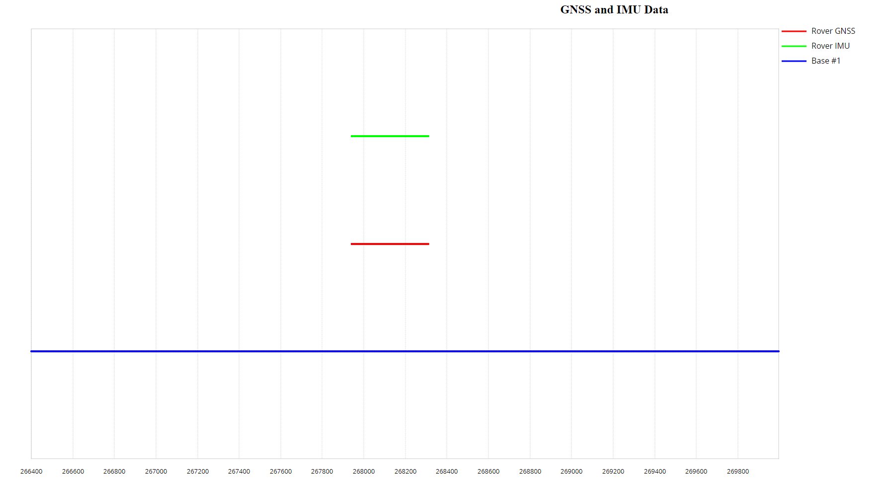
This plot displays the coverage of Rover GNSS, IMU, and Base Station GNSS data. It is crucial to check if the timelines of all three data streams align, if the update rates are as expected, and if there are any gaps in the data. Ensuring complete and synchronized coverage is essential for accurate post-processing.
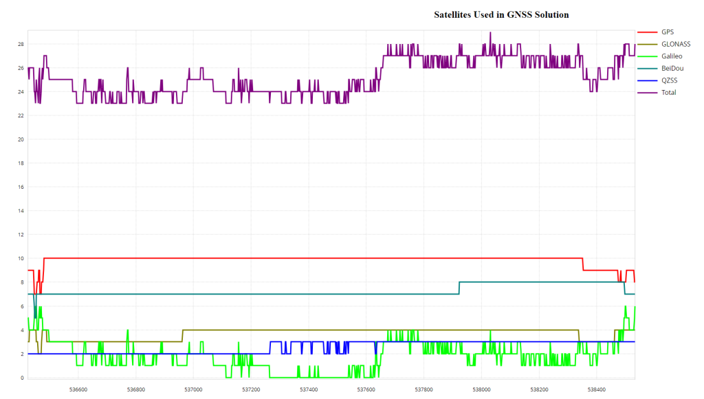
This plot shows the number of satellites used in the solution over time, differentiating between GPS, GLONASS, BeiDou, Galileo, QZSS satellites, and the total number of satellites. It helps in assessing the satellite visibility and availability during data collection, which can affect the quality of the positioning solution.
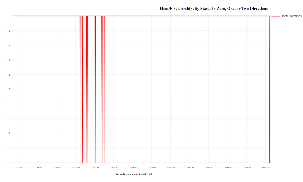
This plot indicates the GNSS carrier phase ambiguity resolution status during processing. It shows:
2: Both forward and reverse solutions achieved an integer fix. This is the desired value for the best GNSS quality.
1: Either the forward or reverse solution achieved an integer fix, but not both.
0: Neither direction achieved an integer fix, resulting in a float solution. If the solution is float (0), lever arm calculations and further IMU-GPS misclosure plots will not be generated as the inherent error associated with the Float is bigger than the error in the lever arm.
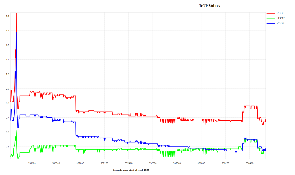
DOP is a dimensionless number that reflects the contribution of satellite geometry to errors in position determination. Lower DOP values indicate better satellite geometry and, consequently, more accurate positioning. Values less than 1 are ideal, representing optimal conditions.
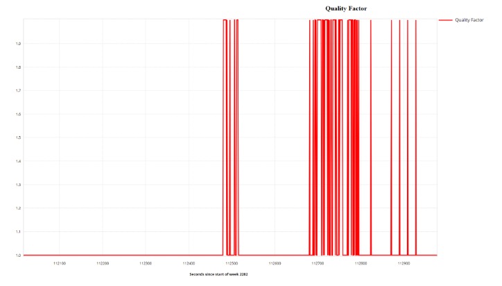
Assigned by Inertial Explorer (IE), the Quality Factor is a dimensionless number ranges from 1 to 6 and indicates the stability of the solution. This combined with the Float/Fix Ambiguity plot serves as a powerful QA/QC check for the trajectory.
1 or 2: Indicates a stable solution, including carrier phase processing. These values represent the best GNSS quality in the trajectory.
3 to 6: Indicates lower quality, only utilizing code phase processing
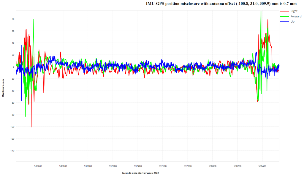
This plot shows the difference between the GNSS solution and the mechanized INS positions obtained from GNSS/INS processing. The plot iteratively improves as lever arm values are refined. Large spikes may indicate an unstable INS solution, while values nearing zero confirm a good GPS solution. This plot is not generated if the Fixed/Float Ambiguity plot indicates a float solution.
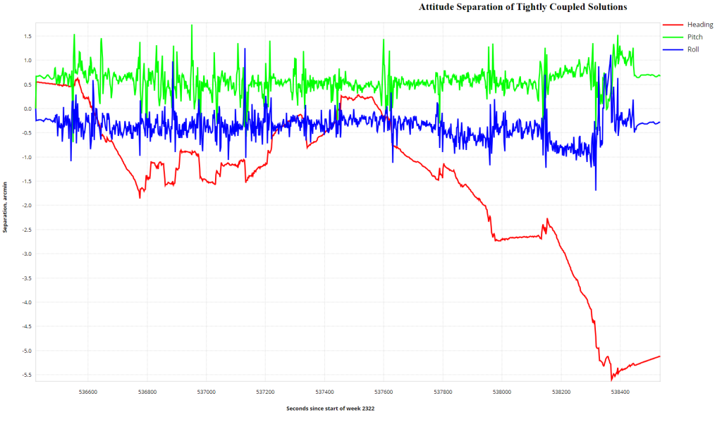
This plot illustrates the difference in roll, pitch, and heading between forward and reverse solutions. Ideally, the separation should be zero, indicating matching solutions. Spikes at the beginning and end are common due to periods of alignment. Larger oscillations in heading are typical and reflect variations in orientation.
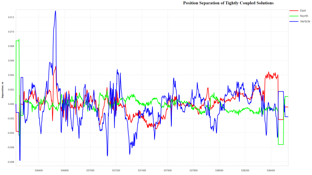
This plot shows the north, east, and height position differences between forward and reverse tightly coupled solutions. Common biases (e.g., inaccurate base station coordinates or residual ionospheric or tropospheric errors) may not be visible in this plot, as they are subtracted out.
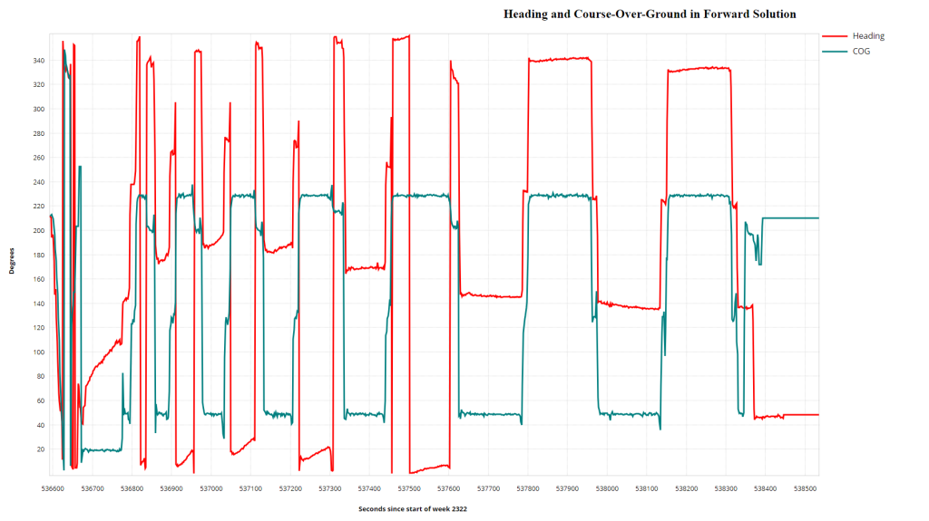
9. Heading and Course Over Ground in Forward/Reverse Solution #
This plot compares the calculated heading as the direction of motion based on GPS calculations. It highlights effects like crabbing and shows any transitions between 359 degrees and 0 degrees as vertical lines. Proper alignment of these plots depends on the correct input of orientation angles in the RESEPI GUI before processing. This plot does not directly affect the absolute accuracy of the point cloud but can be adjusted in PCMasterPro software post-processing.