

SurveyPro Tools Guide and Breakdown #
This dialogue is only available to users with a SurveyPro license, activated in the PCMasterProGL Licensing menu. The license provides access to features like ground/non-ground classification, accuracy assessments, debiasing, DEM generation, and contour creation.
Window Field Entries #
Field entries can be configured to how the user would like. Each tab of the dialogue shows a different step of the SurveyPro pipeline. If only wishing to run a certain step, the user can decide to only check this box and skip other features. After configuring the window to the users processing liking, the Run button may be pressed to processed the selected cloud file.
The user can navigate the dialogue by either selecting individual tabs or using the “Previous” or “Next” buttons.
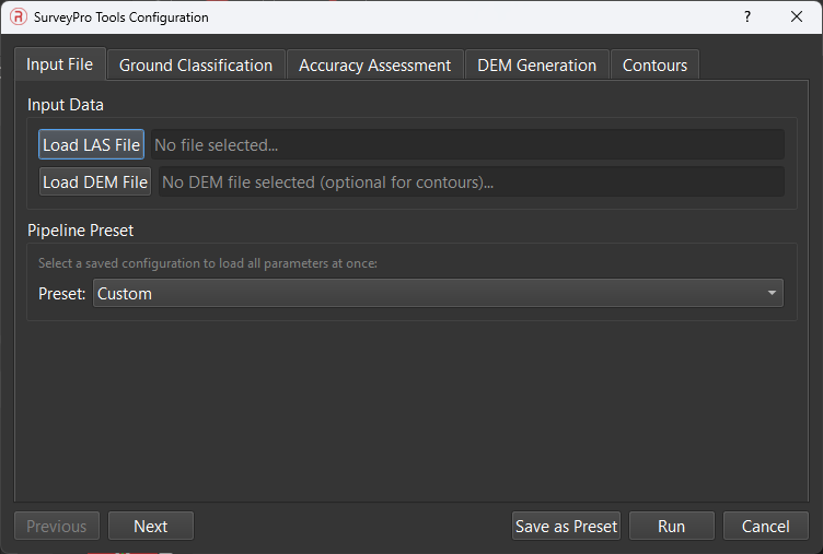
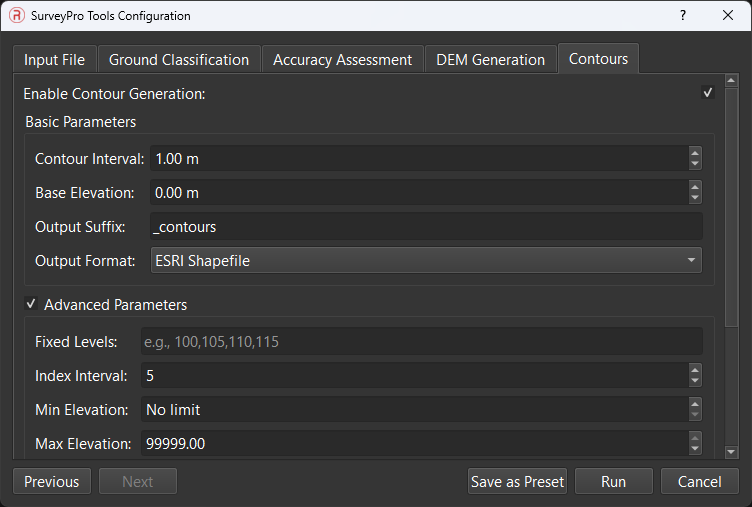
All field entries are in the units of the units related to the cloud file input (ft or m). Ensure all fields are properly entered to account for these changes. GCP’s and cloud files but be in the same vertical and horizontal coordinate frame to ensure a proper assessment. Below shows the configuration menu pop-up when the user selects “SurveyPro Tools” within PCMasterPro.
- Load LAS File – opens File Explorer to allow the user to select the .las file that’s being used for processing. This is necessary for running any of the SurveyPro features besides the contour creation which requires a DEM input.
- Load DEM File – opens File Explorer to allow the user to select the DEM file that’s being used for processing. This is necessary for running contour creation. Users can select an input file or have the DEM used in the current pipeline session.
- Pipeline Preset – Shows a dropdown of the custom preset along with any saved profiles from past runs. These presets can either be set to populate the entire pipeline.
- Previous – Navigates to the previous tab
- Next – Navigates to the next tab
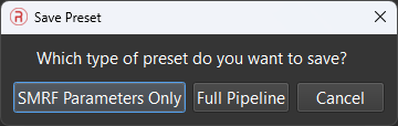
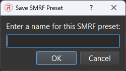
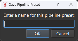
- Save as Preset – Prompts the user to save the currently filled settings as either SMRF only (only ground classification settings) or Pipeline (full workflow). Prompt is followed by a name input. If the user desires to delete a saved preset, find the file named “surveyToolsPresets” within the install directory, open in notepad, and delete the line containing the cooresponding preset name. This file must be saved and PCMasterPro must be restarted for changes to take effect.
- Run – Runs all selected processes and shows current progress in the status window of PCMasterPro
- Cancel – closes the window without running
A settings report is saved at the very start of the run, before any processing happens. This report is saved even if the run later fails.
If you only turn on Contours, and leave classification, accuracy, and DEM off, the tool skips straight to drawing contours from the DEM file you loaded.
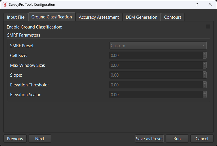
- Ground Classifications Options – checkbox to enable/disable SMRF ground classification. When enabled, points are classified as ground (Classification = 2) or non-ground (Classification = 1) using the Simple Morphological Filter algorithm, which iteratively applies morphological opening operations on an elevation grid to detect bare earth.
- Presets – contains 3 preset profiles for different cloud sceneries or custom option for user defined settings saved as presets.
- Cell Size – defines the cell size (in meters) of the elevation grid used for morphological operations. Smaller values preserve more terrain detail but require higher-resolution input data and significantly increase computation time. This is a fundamental parameter that controls the spatial resolution at which the algorithm analyzes terrain. Typical range: 0.5–5.0 meters depending on data density and terrain detail required.
- Max Window Size – the maximum search radius (in meters) for morphological opening operations. The algorithm grows the window size linearly through successive iterations until reaching this maximum. This parameter must be larger than the largest non-ground feature you want to remove (e.g., building footprint or tall vegetation canopy). If set too small, flat-roofed buildings may be misclassified as ground because the window doesn’t expand enough to “see over” them. Typical range: 12–30 meters.
- Slope – dimensionless scaling factor (rise/run ratio) that controls maximum terrain steepness the algorithm permits during morphological comparisons. A slope of 0.2 means the algorithm permits approximately 1 meter of elevation rise over 5 meters of horizontal distance. In rugged terrain with steep slopes, use higher values (0.3–0.5); on flat terrain, use lower values (0.1–0.2) to aggressively remove vegetation and structures. Typical range: 0.1–0.5.
- Elevation Threshold – maximum vertical distance (in meters) a point can be above the morphologically-smoothed ground surface to still be classified as ground. This is the primary parameter controlling classification sensitivity. Smaller values create stricter classification—the algorithm requires points to closely match the smoothed surface. Larger values are more permissive, accepting points from low vegetation or terrain undulations. This parameter directly controls how many points are classified as ground. Typical range: 0.3–1.0 meters.
- Elevation Scalar – scale factor for the elevation.
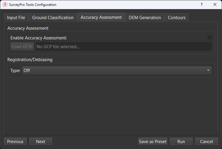
- Accuracy Assessment – checkbox for accuracy assessment.
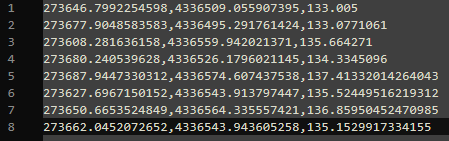
- Load GCPs – this button opens File Explorer for the selection of GCP coordinates. The typical format is Easting, Northing, Ellipsoidal Height. See the example below.
- Registration/Debiasing – checkbox for registration and debiasing in relation to local values or GCPs.
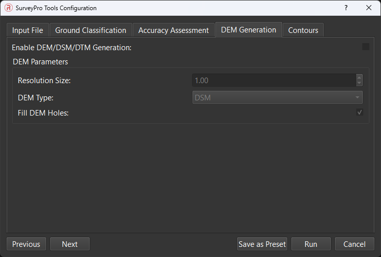
- DEM/DSM/DTM Generation – checkbox for generation of elevation, surface and terrain models
- Resolution Size – defines the size of each pixel in the generated DEM, DSM, or DTM. A smaller resolution creates a more detailed model, while a larger one results in a more generalized representation of the terrain.
- DEM Type – choose between a DSM or DTM
- Fill DEM Holes – attempts to fill in areas where no points are collected with estimated point spreads. This helps with random blank spaces caused by using ground classified points for DEM creation.
- Contours – checkbox for enabling/disabling the contour generation feature. There must be a DEM input within the Input File tab in order for this toolset to be taken advantage of.
- Contour Interval: Defines the constant vertical distance between consecutive contour lines generated from the source raster.
- Base Elevation: Sets the vertical offset relative to zero from which the contour intervals are calculated.
- Output Format: Determines the geospatial vector driver used to write the output file, such as ESRI Shapefile or GeoJSON.
- Fixed Levels: The start of the advanced settings. Designates a specific list of elevation values to extract as contours, independent of the standard interval generation.
- Index Interval: Sets the periodic interval at which “major” contours are categorized, often used to differentiate line weights in cartography.
- Min Elevation: Establishes the lower elevation threshold, excluding any source data below this value from the contour generation process.
- Max Elevation: Establishes the upper elevation threshold, excluding any source data above this value from the contour generation process.
- Layer Name: Specifies the internal name assigned to the vector layer within the output dataset.
- Elevation Field: Defines the name of the attribute column where the calculated elevation value for each contour geometry is stored.
- ID Field: Defines the name of the attribute column used to store a unique numerical identifier for each contour feature.
- NoData Value: Identifies the specific pixel value representing missing or void data in the source raster so it can be ignored during processing.
- Precision: Controls the number of decimal places used when writing the elevation values to the output attribute table
Common Workflows #
Sort Ground and Non-Ground Points Only #
1. Load your LAS file.
2. Turn on Ground Classification .
3. Pick a preset ( Flat Urban Area , Mountainous Terrain , or Forest or Complex Terrain ). Or set the five values yourself. See Section 5.
4. Leave Accuracy, DEM, and Contours off.
5. Press Run .
6. You get a new file named `<yourfile>_processed.las`. Ground points are marked in the Classification field.
Check Accuracy Against Survey Points #
1. Load your LAS file. Turn on Ground Classification . The accuracy check only looks at ground points. If you skip classification, the check only works if your LAS file was already classified before.
2. Load your GCP file. Match the X, Y, and Z columns in the dialog that appears. See Section 4.
3. Leave Registration set to Off .
4. Turn on Accuracy Assessment .
5. Press Run .
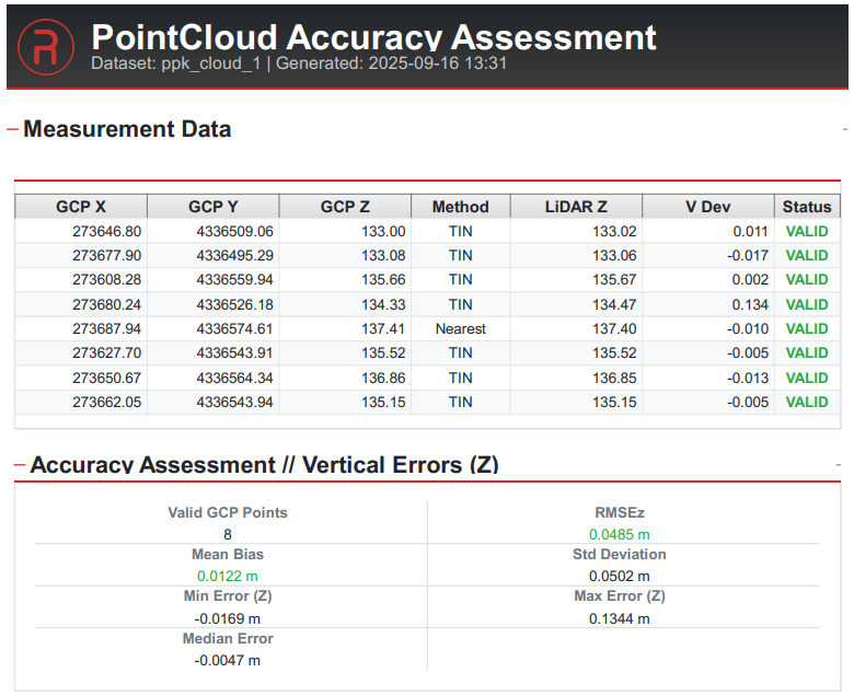
6. You get an accuracy report named `<yourfile>_accuracy_report.pdf`. This report shows accuracy before any correction, and it is the only report you get in this workflow.
Automatically Correct Height Errors #
1. Follow the steps in 3.2 first. Once you load a GCP file, the Automated Averaged RSMEz option turns on in the Registration list. It stays off until a GCP file is loaded.
2. Choose Automated Averaged RSMEz .
3. Press Run . The tool checks accuracy, works out the average height error, and shifts the point cloud up or down to fix it. It skips the correction if the error is 1 cm or less.
4. Your final report shows the accuracy after correction, not before. If you want to know the error before correction, watch the on-screen progress messages during the run — that value is not saved anywhere else.
5. The saved LAS file already has the height correction applied.
Manually Correct Position or Orientation #
1. Choose Manual in Registration. A 4×4 grid appears, starting as an identity matrix (no change).
2. Type in your own transform values. The last column of the first three rows holds the X, Y, and Z shift.
3. Press Run .
4. Important: if Accuracy Assessment is also on, the report shows accuracy before your manual correction, not after. To check accuracy after a manual correction, run the tool a second time on the `_processed.las` file, with Registration set to Off .
Build a Terrain Model (DSM or DTM) #
1. Load your LAS file. If you want a DTM , run Ground Classification first. A DTM only uses ground points. Without classification, there are no ground points to use, and the DTM comes out empty.
2. Turn on Digital Model Generation .
3. Set the pixel size ( Resolution ) and choose DSM or DTM .
4. Optionally turn on Fill DEM Holes . This smooths small gaps. It does not fill large gaps.
5. Press Run .
6. You get a file named `<yourfile>_dsm.tif` or `<yourfile>_dtm.tif`.
Draw Contour Lines #
Option A — right after building a DEM in the same run:
1. Turn on Digital Model Generation, as in 3.5.
2. Turn on Contours . Set the interval and format. See Section 5.
3. Press Run . Contours are drawn from the DEM this run just built.
Option B — from a DEM file you already have:
1. On the Input File tab, load your existing DEM file (a `.tif` file).
2. Leave Ground Classification, Accuracy, and DEM Generation off.
3. Turn on Contours .
4. Press Run . The tool skips LAS processing and draws contours straight from your DEM file.
The contour file is saved next to the DEM, named after the DEM or LAS file plus your chosen suffix.
Full Pipeline, Start to Finish #
This example runs everything in one pass: classify ground points, auto-correct height, build a DTM, and draw contours.
1. Load your LAS file and GCP file.
2. Turn on Ground Classification and set your SMRF values.
3. Turn on Accuracy Assessment. Set Registration to Automated Averaged RSMEz .
4. Turn on Digital Model Generation. Set DEM Type to DTM .
5. Turn on Contours.
6. Press Run . The tool follows the order in Section 2: classify, check accuracy, correct, check accuracy again, save the LAS file, build the DTM, then draw contours.
GCP File Format #
– Use a plain text file. Columns can be separated by commas or spaces.
– Any line starting with `#` is treated as a comment and ignored.
– Columns can be in any order. When you load the file, a dialog lets you say which column holds X, Y, and Z.
– You can tell the tool to skip a number of header rows (0 to 10).
– Rows with too few columns are skipped without an error message.
– The tool does not convert units or coordinate systems. Your GCP file must already use the same coordinate system and height reference as your LAS file.
Example file:
“`
# GCP_ID, Easting, Northing, Height
GCP01, 512340.12, 4187650.44, 231.885
GCP02, 512410.87, 4187722.10, 229.410
“`
For this file, set X to column 1, Y to column 2, Z to column 3, IDs are Column 0.

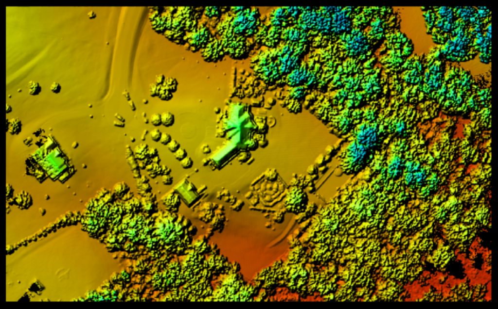
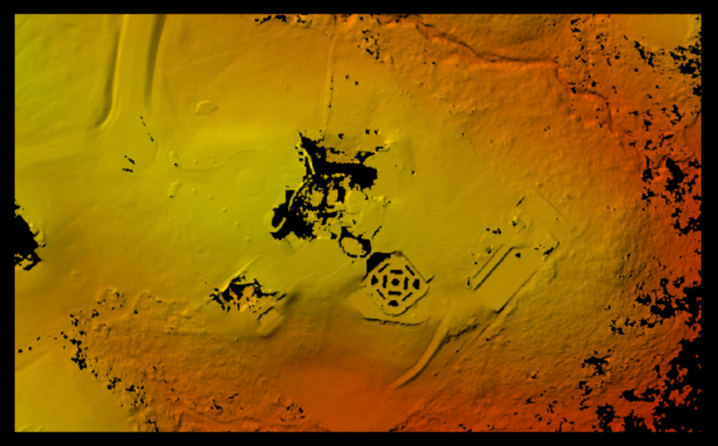
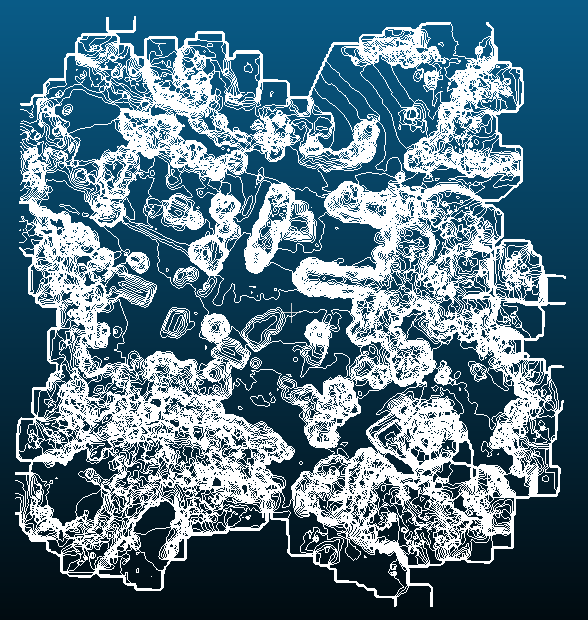
To observe the entire process in practice, we suggest viewing the video recording below.