Orthomosaic is a commonly implemented geospatial deliverable created using images. This guide will show how to retrieve these models from images from RESEPI in PIX4D Mapper by PIX4D. We will also look at the key aspects to pay attention to.
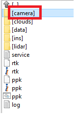
After processing LiDAR data in PCMasterPro, the project folder will look like this, Figure 1.
Figure 1. “Add Data” workflow.
We are interested in the folder with photos called “Camera.” It contains all the photos obtained during the data recording process. It is also important to have a file with Ground Control Points for georeferencing. The more accurately the GCPs are measured, the more accurate the orthomosaic georeferencing will be.
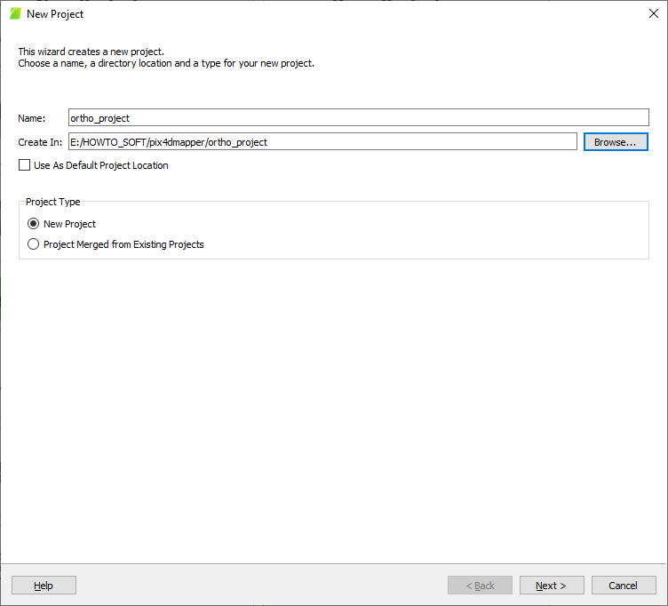
To generate an orthomosaic, you need to create a project and import images. To do this, click the “New Project…” button in the program’s start window, as shown in Figure 2. Another option is to use the “Project” -> “New Project…” menu, as shown in Figure 3.
Figure 2. “Open LAS file” window and tabs.
Figure 3. Creating a project via menu items.
After this, the window shown in Figure 4 will open. Here you need to specify the project name and the path to which the project will be saved. There is a choice to use the specified default path for all the following projects, and also to select the project type:
New Project
Project Merged from Existing Projects
Figure 4. Name and path to project files.
Setting the project type allows the user to do the following:
In the first case (“New Project”) a new project is created.
In the second case (“Project Merged from Existing Projects”) the user can merge projects created using different types of capturing, for example, ground and aerial. Or merge several projects that were separated due to limited computing resources.
We will be creating a new project from scratch, so we leave this parameter by default, i.e. “New Project”. After we have set the path and name, click “Next >”.
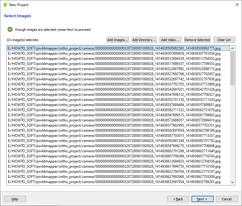
The window will look like the one shown in Figure 5. The following functions are available here:
“Add Images…”. The function imports the selected images from the specified path.
“Add Directory…”. The function imports all images from the specified directory from the specified path.
“Add Video…”. The function imports videos.
“Remove Selected”. The function removes the selected data from the list.
“Clear List”. The function clears the entire list of data.
Figure 5. Importing images.
We will use the directory import. To do this, click on “Add Directory…” and select the path to the folder with images. As a result, the photos from the directory will be displayed in the list of images, as shown in Figure 6.
Figure 6. List of images.
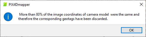
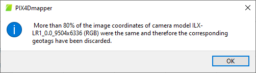
Click «Next >». The program will start reading EXIF information from the images. After this, an information message will be displayed, as shown in Figure 7. We will use control points for georeferencing, so just click «OK».
Figure 7. Information message.
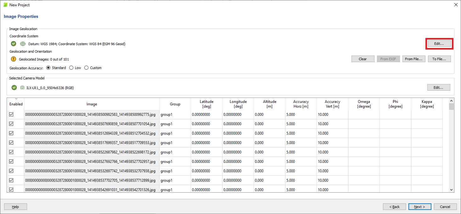
By default, the program automatically determines the coordinate system and camera model. The camera used in RESEPI is in the PIX4D Mapper database, i.e., there is no need to make changes.
However, it is important to pay attention to the coordinate system; although images are geotagged with EXIF data, the coordinate system may not be understood correctly by the software.
Figure 8. “Image Properties” window.
Therefore, we should do the following:
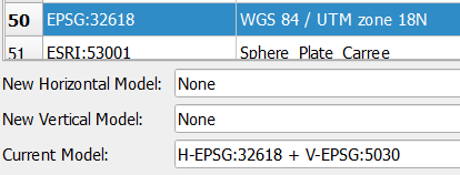
For example, in this case, our project uses the parameters shown in Figure 9. As we can see, WGS84/UTM is used, and “Height above the WGS84 ellipsoid” is used for the height model.
Figure 9. Project coordinate system in PCMaster.
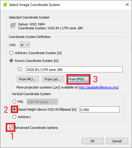
Therefore, we click on “Edit…”. The window shown in Figure 10 will open. Here, according to the order marked with numbers, check the box next to “Advanced Coordinate Options” 1. Then select the vertical model “Geoid Height Above WGS 84 Ellipsoid [m]” 2. Click on “From EPSG…” 3, and select the horizontal model EPSG:32618 (these settings may differ for your project!) from the list of available models. Then click “OK”.
Figure 10. Setting up the source coordinate system for images.
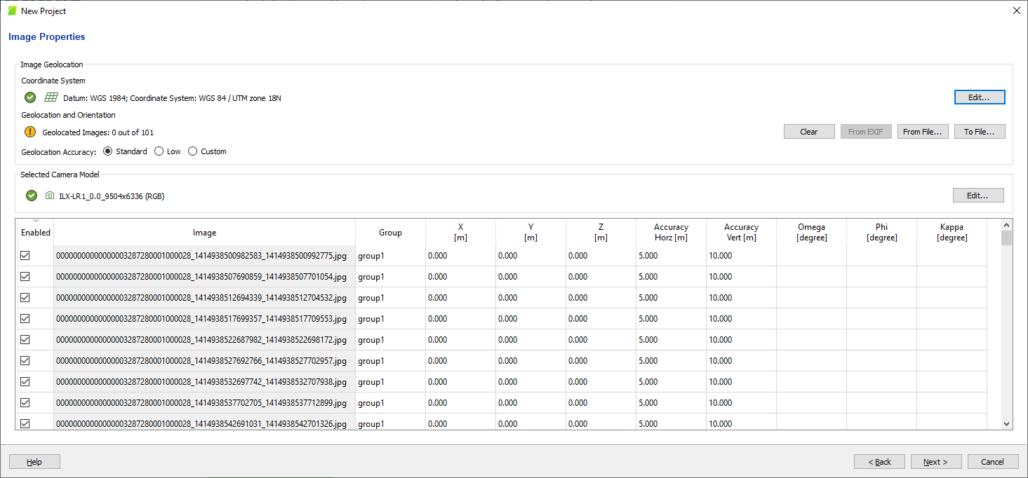
After the coordinate system has been correctly set up and the list of images has been loaded, the project settings window will look like Figure 11. Now the coordinate system is set correctly.
Figure 11. The configured coordinate system.
Click “Next >” to apply the settings. The program will again display the information message shown in Figure 12. Click “OK”.
Figure 12. Information message.
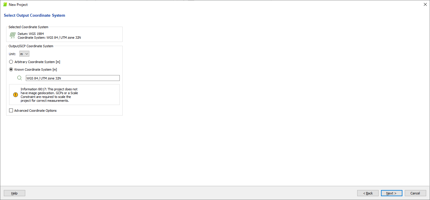
The program will prompt you to select a coordinate system for orthomosaic, Figure 13. Repeat the procedure as described above. But if you want to get orthomosaic in a different coordinate system, then select the appropriate parameters here. We will use the same coordinate system. After setting up, click “Next >”.
Figure 13. Output Coordinate System Setup.
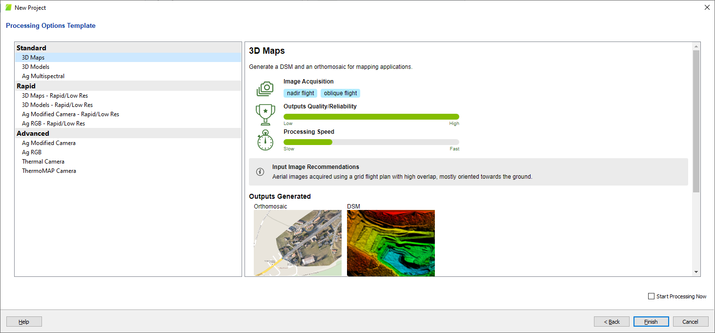
The program will prompt you to select a template for data processing, Figure 14.
Here we select “3D Maps” and click “Finish”.
Figure 14. Selecting a template for data processing.
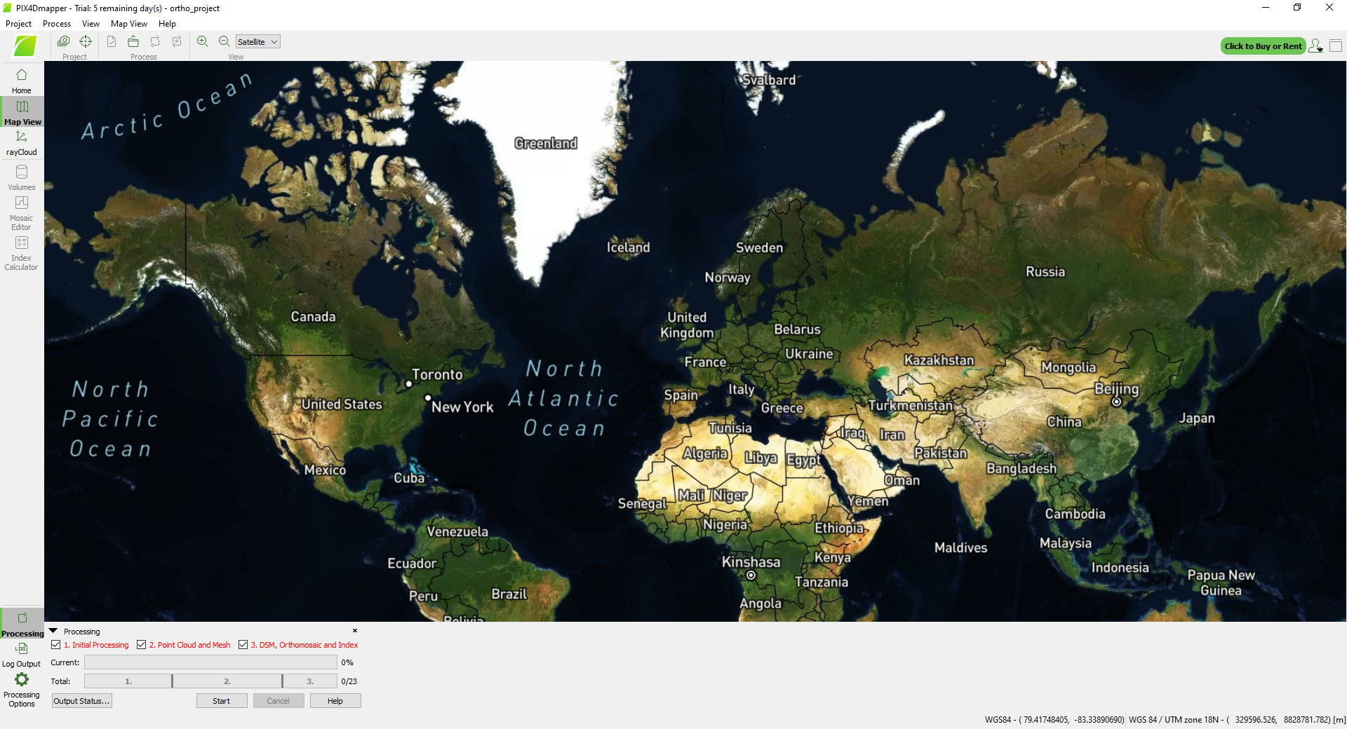
After selecting a template, the main program window will look like this, Figure 15.
Figure 15. The main program window after setting up the project.
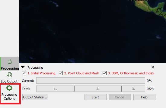
Before starting processing, we need to set up the processing process. To do this, in the lower left corner, click on “Processing Options”, in Figure 16.
Figure 16. Processing Options menu.
The window shown in Figure 17 will open. In it, you can immediately set up all 3 stages of processing, but since our photos do not have georeferencing, in this case, the processing procedure will be divided into several stages.
For now, we are only interested in the first stage “Initial Processing”. Therefore, we uncheck “Point Cloud and Mesh” and “DSM, Orthomosaic and Index”. We will return to stages 2 and 3 later.
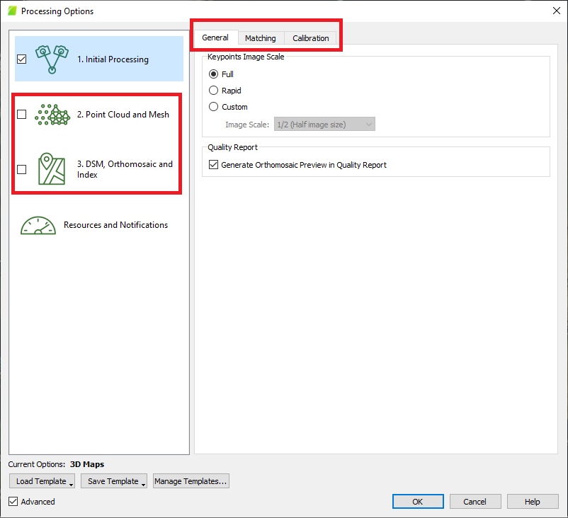
Figure 17. Processing Options.
The “General”, “Matching”, and “Calibration” tabs have additional processing parameters, which we set by default.
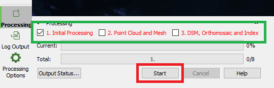
Click “OK”. The window will close and now only the first processing stage will be selected in the lower left corner, as shown in Figure 18.
Figure 18. Settings for initial processing.
Click “Start”. Processing will begin, which may take some time depending on the computational power of your PC.
After the process is complete, a window with a report will open, which is of little interest to us now, since we have not yet added control points for georeferencing. Therefore, we close it and proceed to add control points.
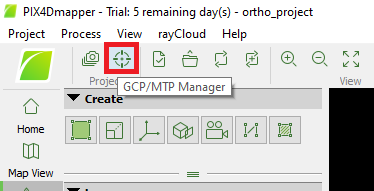
To add control points, you need to click on the icon with a crosshair in the upper left corner of the main program window, Figure 19.
Figure 19. GCP/MTP Manager.
The window shown in Figure 20 will open.
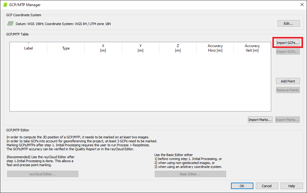
Figure 20. «GCP/MTP Manager» window.
• We will use a file with control points, so click on “Import GCPs…”. The import window shown in Figure 21 will open. From the drop-down list “Coordinates Order” you can select the order of coordinates: X, Y, Z (or Latitude, Longitude, Altitude) or Y, X, Z (or Longitude, Latitude, Altitude). This should be taken into account when importing.
Figure 21. Control points import window.
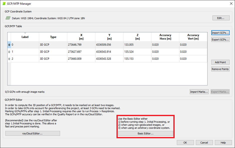
Click on “Browse…” and specify the path to the file with control points. Then click on “OK”. As a result, we will see a list of our control points, as shown in Figure 22.
Figure 22. Control points list.
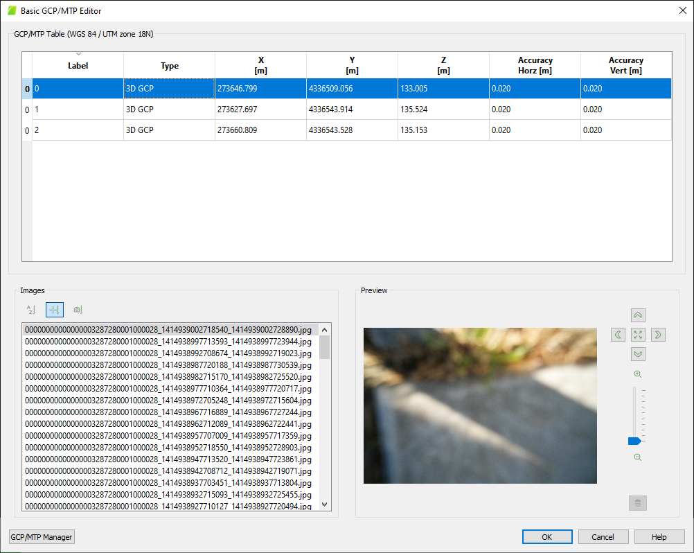
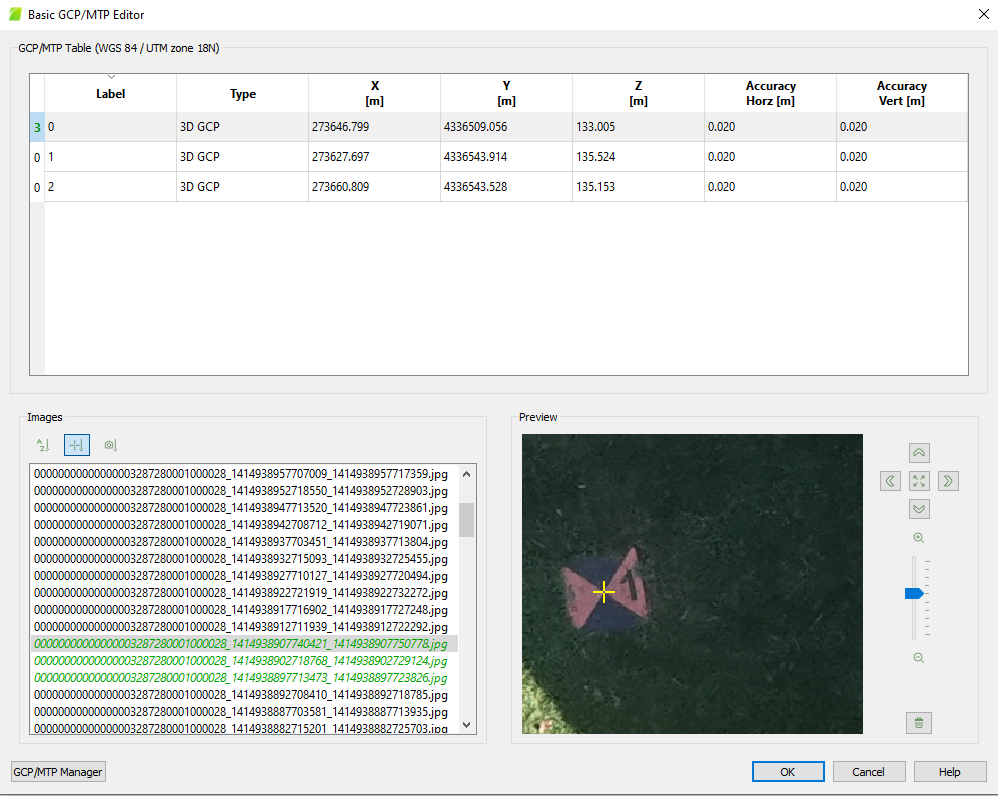
Click on “Basic Editor …”. The “GCP/MTP” Manager window will look like Figure 23.
Figure 23. Basic control point editor.
Here you need to select 2-3 photos with the corresponding marker for each control point. For example, we know that the first checkpoint corresponds to target number 1. Click on the first checkpoint in the list, then on the image in the image list, and look for the target in the image (if necessary, you can zoom in and move the image). It is enough to mark 2-3 images where the target is found. Click in the center of the target with the left mouse button (we recommend zooming in on the image so that the click is in the center of the target). A yellow cross will appear, in Figure 24.
Figure 24. Basic control point editor.
Repeat the procedure for the remaining control points. Then click “OK”.
After that, select the “Reoptimize” tool in the program menu, Figure 25. This tool is needed for geolocating our data.
Figure 25. “Reoptimize” tool.
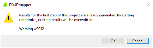
A warning window will open, as shown in Figure 26. Click “OK”. A status bar will appear in the lower left corner. After the process is complete, the program window will look like Figure 27.
Figure 26. Warning window.
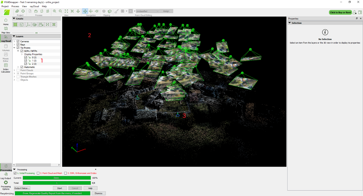
Figure 27. The program window after binding data to control points.
Control points will be visible in the drop-down list with layers 1, and blue and green markers 3 will appear in the data display window 2. The calculated position of the control point is displayed on the images as a blue circle with a dot in the middle, while the green marker is the coordinates of the control point from the file. After marking the control point on 2 images, a green cross appears on all images. The green cross is a reprojection of the proposed 3D point, and its location depends on the marks already made for the reference point.
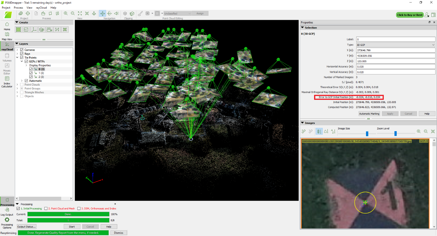
Click on the first control point in the drop-down list of control points. Information about the accuracy of the reference, as well as photos with markers, will be displayed on the right in the properties, as shown in Figure 28.
It is important to pay attention to the accuracy of “Error to GCP Initial Position [m]”. As you can see, it is within 4 cm for X, Y, Z. Approximately the same result was obtained for the remaining points.
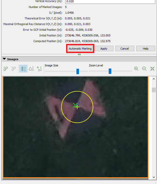
As we remember, in the basic editor we selected only 3 photos for georeferencing. In order for the program to calculate the georeferencing more accurately, we will use automatic marking of targets, Figure 29.
Figure 28. Selected control point and its parameters.
Click on the control point from the dropdown list, click “Automatic Marking” and wait for the marking process to complete. Then click “Apply” to save the changes. Repeat the process for all control points.
Figure 29. Automatic target marking.
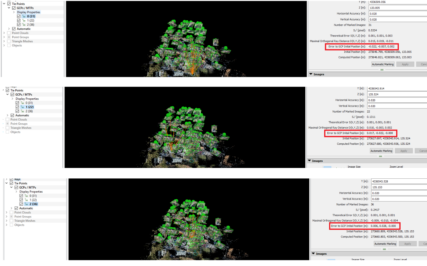
After the program has marked all targets, select the “Reoptimize” tool again. After the process is complete, we can see an increase in accuracy, Figure 30. Compare Figures 28 and Figure 30. For the first control point, the accuracy has increased by about 1 cm, for 2 and 3, an increase in the accuracy of the binding is also noticeable. Now the accuracy of the georeferencing is within 3 cm for all points.
Figure 30. Increasing accuracy after marking all targets.
After georeferencing the data, we can start processing the data to generate Orthomosaic.
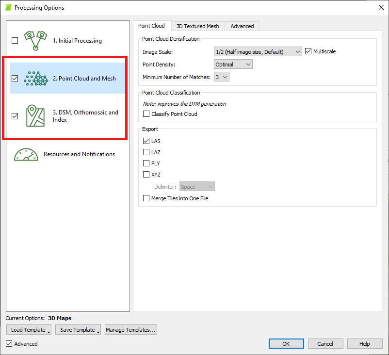
To do this, click on “Processing Options” in the lower-left corner of the main window and uncheck “Initial processing”, and check the boxes next to “Point Cloud and Mesh”, and “DSM, Orthomosaic and Index”, as shown in Figure 31. Set the processing parameters by default. Click “OK”.
Figure 31. Processing Options.
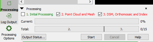
The window will close. Now we will see that the second and third stages are selected, as shown in Figure 32. Click “Start” and wait for the processing to complete.
Figure 32. Processing parameters for generating Orthomosaic.
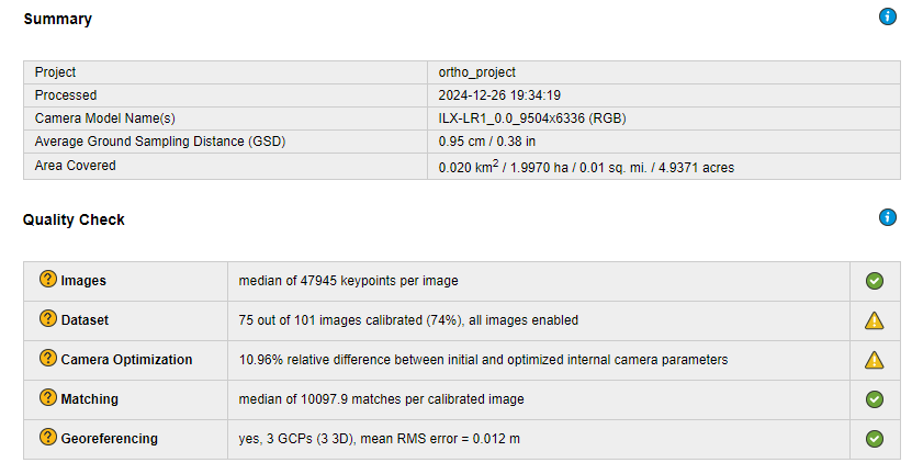
A report will open automatically during processing. Now we can see the results of georeferencing accuracy as well as Average GSD as shown in Figure 33. As you can see, we got a great result, GSD is less than 1 cm and RMS of georeferencing is less than 1.5 cm.
Figure 33. Quality Report.
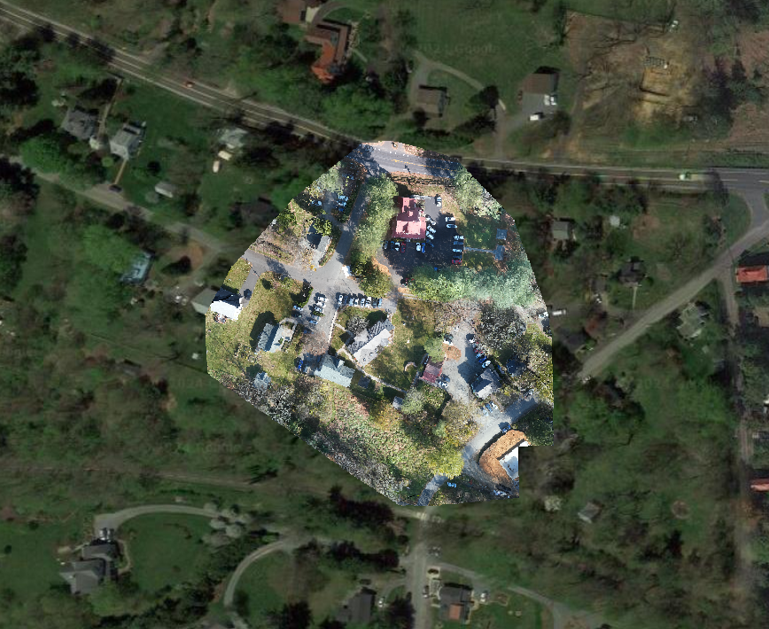
As a result, we got orthomosaic with accurate georeferencing which we superimposed on Google Maps Figure 34.