An aerial and ground survey can obtain a full terrain scan. Most often, aerial surveys are carried out using GNSS, which results in georeferenced data after the flight. The ground part is often scanned in SLAM mode. Thus, the ground scan data has local coordinates. To combine both datasets, georeferencing of SLAM data is necessary. And this can be a big problem, especially for beginners of LiDAR payloads. But in fact, it is very simple. This guide will show how to georeference SLAM point cloud data from RESEPI in TerraScan by Terrasolid. In this case, the Spatix platform was used, but this tutorial will be useful when using the Microstation platform from Bentley Systems Inc. as well. We will also look at how to generate reports and show you the key aspects to pay attention to.
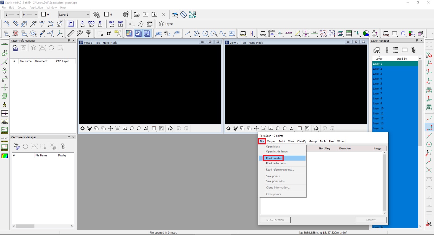
Any activity with point clouds begins with the import of data. Create a new CAD file, then click on “File” -> “Read points…” in the menu, as shown in Figure 1.
Figure 1. Open data file.
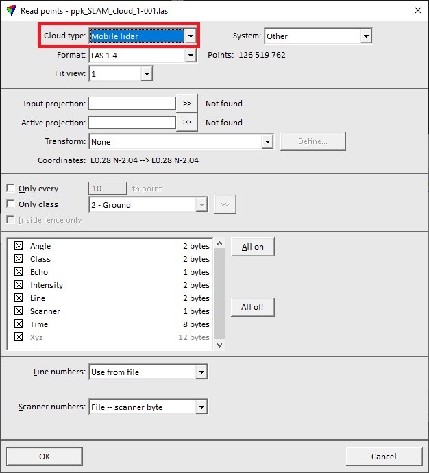
After that, a window will open where you can select the path to the point cloud file. Select the desired point cloud and click “Open”. This will open the standard data import window shown in Figure 2. As you can see, in this case, the coordinate system is not defined, because SLAM data has a local coordinate system. Here it is important to choose the correct type of point cloud, as this is recommended to optimize the processing speed for many automatic procedures. In this case, we will process SLAM data that were recorded by a mobile lidar, so we select “Mobile Lidar” in the drop-down list. Let’s leave the other parameters unchanged and click on “OK”.
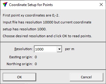
The window shown in Figure 3 will open, in which we set the resolution according to the resolution of the current coordinates. In this case, the resolution is set to 1000. After that, we click on “OK”. The import process will begin, and it may take some time.
Figure 2. Data import parameters.
Figure 3. Selecting the resolution of the point cloud.
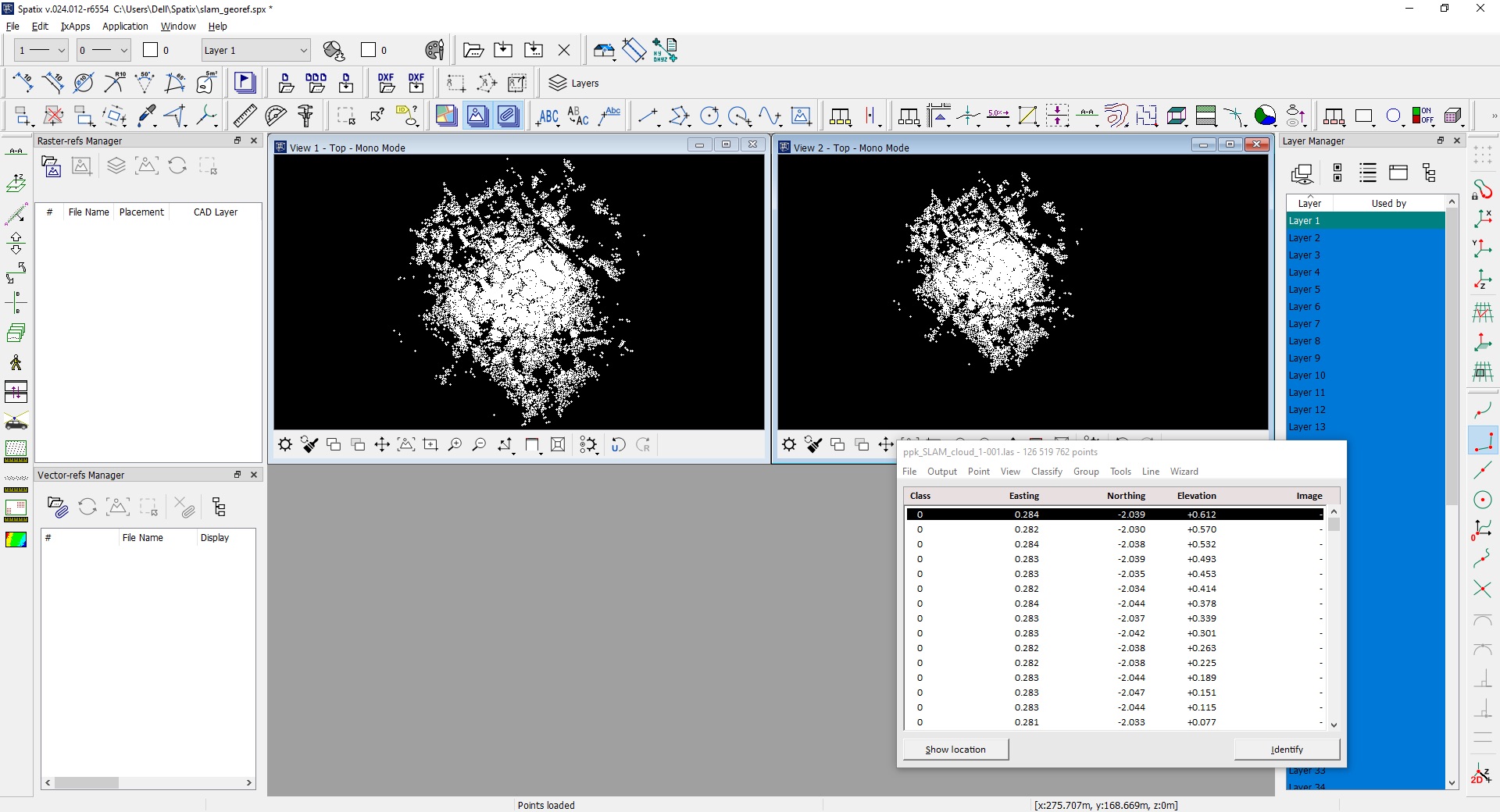
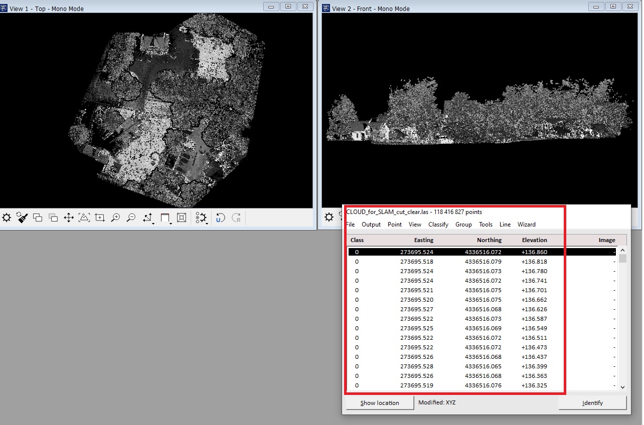
After the upload process is complete, the main window of the program will look as shown in Figure 4. As you can see, the Terrascan window automatically displays a list of points where you can find out the coordinates of the point and the class it belongs to. By default, all points are unclassified and belong to the general class “Class 0”.
Figure 4. Main program window after point cloud loading.
After loading we can continue our work, and now we will tell you how to process the point cloud before georeferencing.
For further work, we will need to familiarize ourselves with the classification procedure, but first, we will cut off the unnecessary areas in our point cloud. To do this we will need to:
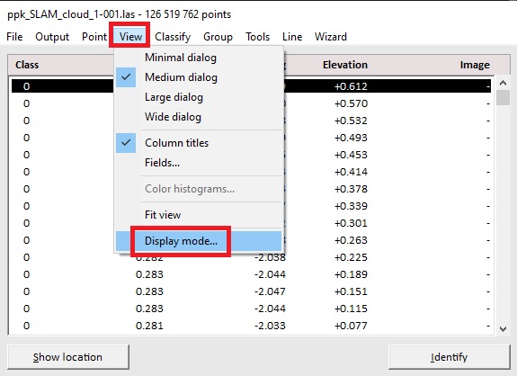
Click on the menu “View” -> “Display mode” and change the color of the unclassified cloud to something other than white, Figure 5.
Figure 5. Display options.
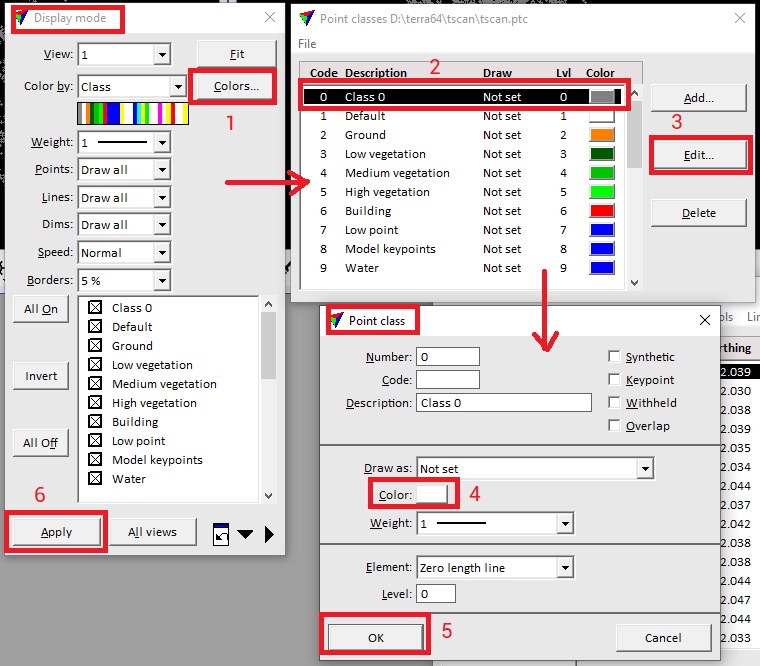
This will open the “Display mode” window where we click on “Colors” 1, Figure 6.
This opens the “Point classes …” window where you select the class whose color you want to replace 2 and click on “Edit” 3.
The “Point class” window will open in which you click on the color next to the “Color” field 4 and change it, for example, to gray. After changing the color, click on “OK” in the “Point Class” window. This will close it.
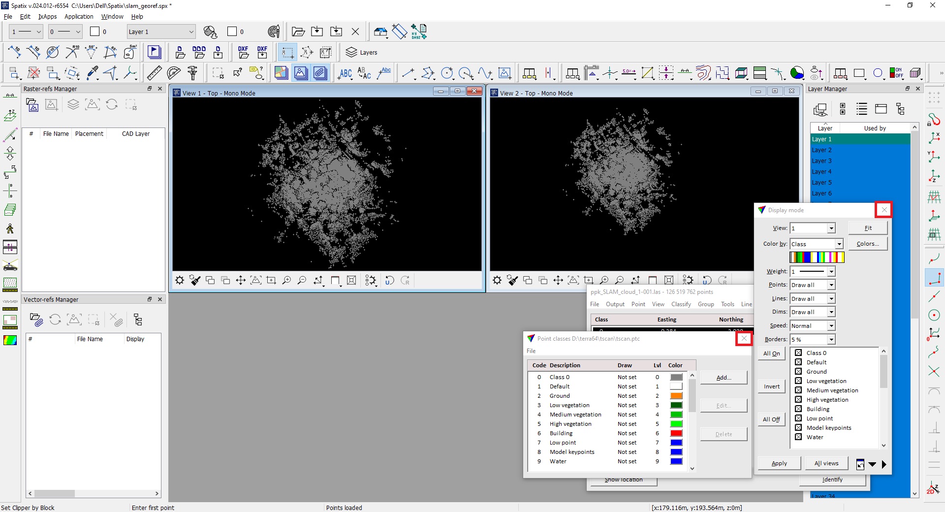
Click on “Apply” in the “Display mode” window and the point cloud will be colored as shown in Figure 7.
Figure 6. Changing the color of an unclassified point cloud.
After that the windows can be closed by clicking on the cross in the upper left corner.
Figure 7. Changed color for the unclassified point cloud.
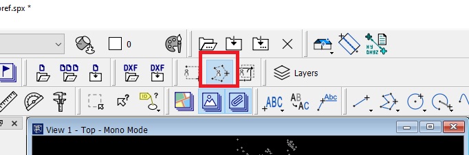
Now we can remove unnecessary points using the clipping tool in the toolbar.
We’re going to use clipping by polygon, so click on “Set clipper by polygon” in the toolbar, Figure 8.
Figure 8. The clipping tool.
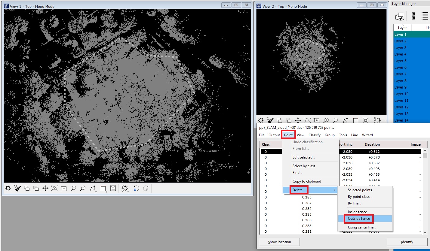
Select the desired area. To do this, click on the point cloud and draw a line to the boundaries of the desired area we want to select. Then click on “Point” -> “Delete” -> “Outside fence”, as shown in Figure 9.
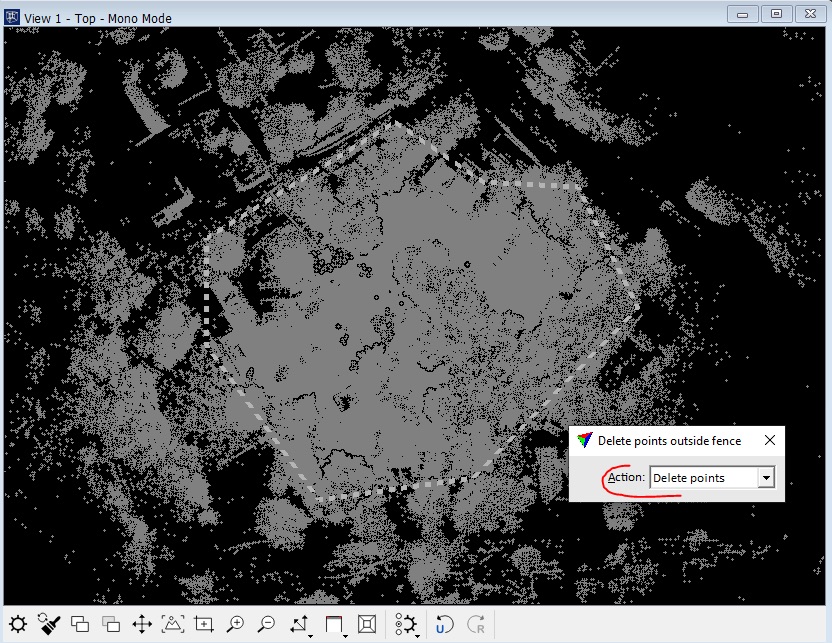
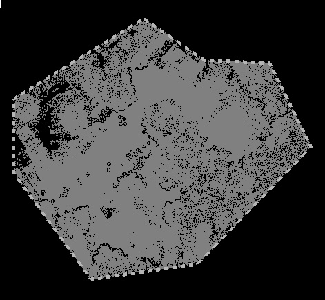
The “Delete points outside fence” window will open, Figure 10. Then click anywhere on the point cloud to accept the changes. As a result, the points that are located “outside” the selection area will be deleted, as shown in Figure 11.
Figure 9. Menu for deleting points outside the selection area.
Figure 10. Selected area for deleting points.
Figure 11. The point cloud after deleting points outside the selection.
As you may have noticed, the lines that are displayed during the selection process are white. Since the point cloud is unclassified by default and is also white in color, the lines would not be visible when defining the area. So, we immediately changed the color of the cloud for convenience.
Now we can move on to preparing the point cloud for SLAM georeferencing.
To do this, let’s display the cloud from the side view. To do this, you need to:
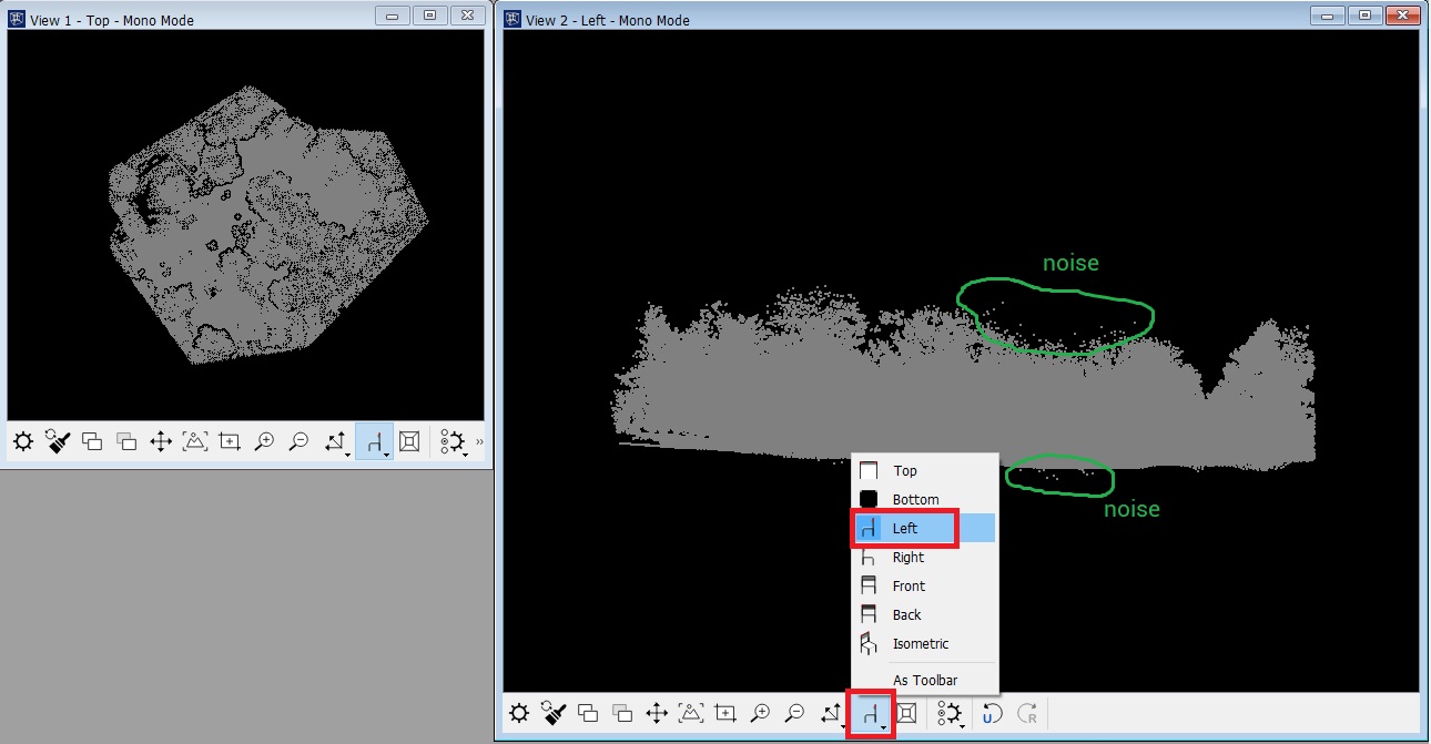
In the toolbar of the second view window (you can use the first one if you want, but we’ll leave it for viewing the cloud with a top view), click on the change view icon.
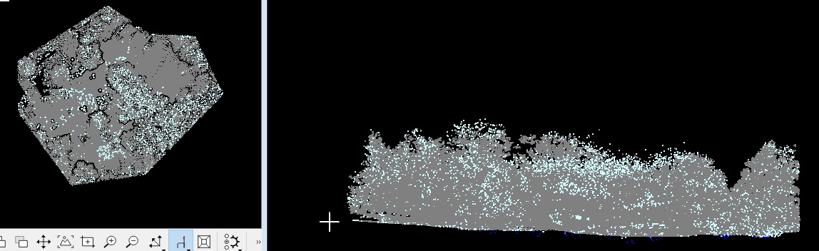
Click on the side from which we want to view the point cloud. In this case, we choose “Left” and click on the point cloud, as shown in Figure 12. It will then be displayed with a side view. As you can see there is some noise in the point cloud, which must be removed.
Figure 12. Change the view of the point cloud in the second view window.
To remove the noise, we can use the same tool we used earlier – “Set clipper by polygon” or we can use classification to automatically detect the noise. In this case, we will use the classification.
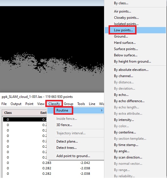
In the menu “Classify” -> “Routine” selects the desired type of classification. First, we will remove the points that are below the surface level, i.e., at the bottom of the point cloud. To do this, click on “Low points…”, Figure 13.
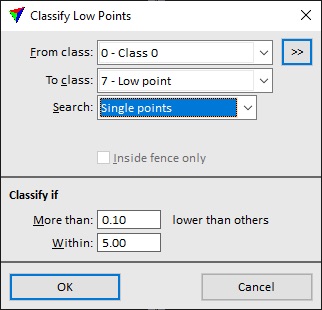
A window with classification parameters will open, as shown in Figure 14. In this window, you need to adjust the parameters, as they are essential for accurate classification.
Select the desired class “Class 0” from the drop-down list. The program has automatically selected the class to which the points “7 – Low Point” will be assigned.
In this case we will search for single points that are farther than 0.1 m from the other points, so change the parameter next to the “More than:” field to 0.1 meters. Click “OK”.
Figure 13. Classification menu.
Figure 14. Classification parameters for "Low Points".
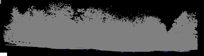
As a result, the noise that is “under the cloud” is classified as a “Low point”. The program automatically highlighted them in a different color (blue) for clarity, Figure 15.
Figure 15. The noise is classified as "Low Points".
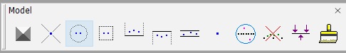
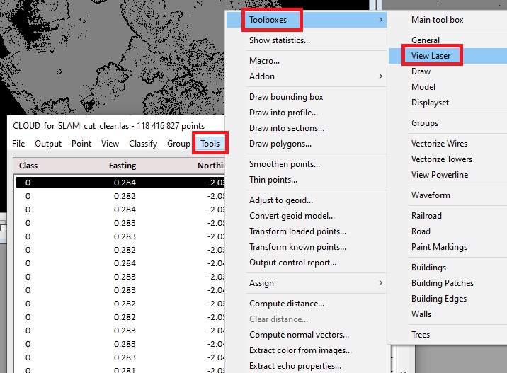
If after the “Low point” classification in automatic mode there are points that can also be classified as “Low point”, but they were not determined by the program (this is due to the parameters), then they can be conveniently and quickly deleted manually. To do this, you will need the toolbox, which is available from the menu “Tools” -> “Toolboxes” -> “Model” in the Terrascan window. The appearance of the toolbox toolbar is shown in Figure 16.
Figure 16. Appearance of the "Model" toolbox toolbar.
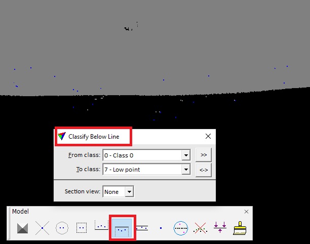
Click on the icon shown in Figure 17 to select the “Classify Below Line” tool. In the window that opens, select the class whose points will be placed in “Low Points”.
Figure 17. Selecting the "Classify Below Line" tool and setting the classification parameters.
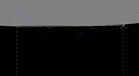
After that, draw a line over the points that we want to classify, as shown in Figure 18. Click in the desired place in the point cloud to confirm the operation.
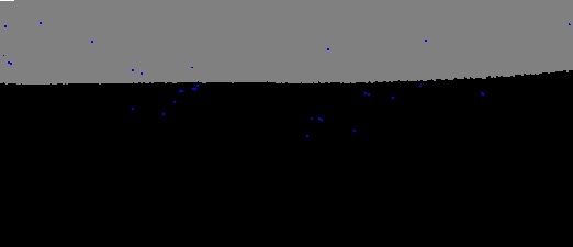
The points under the line will be classified as “Low Points”, as indicated by the color of their selection, as shown in Figure 19.
Figure 18. Manual selection of points for classification as "Low Points".
Figure 19. The points under the line are colored blue, according to the color of the "Low Points" class.
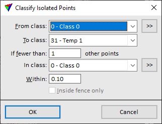
In the same way, we classify the “Isolated Points” with the parameters shown in Figure 20. The result of the classification is shown in Figure 21.
Figure 20. Classification parameters for "Isolated Points".
Remember that for your dataset the appropriate parameters may be different!
Figure 21. Classified “Isolated Points”.
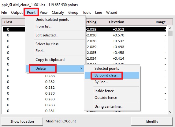
Now we will delete these points using the menu “Point” -> “Delete” -> “By point class…” as shown in Figure 22.
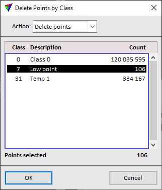
A window will open with the existing point classes, Figure 23. Select “Low point” and click on “OK”. The selected points will be deleted.
Repeat the procedure for the “Temp 1” class.
Figure 22. "Delete by point class" menu.
Figure 23. Selecting the point class to be deleted.
You can repeat the procedure several times with different parameters to achieve the best result. Other classification options are also available, which can also be used for better noise removal.
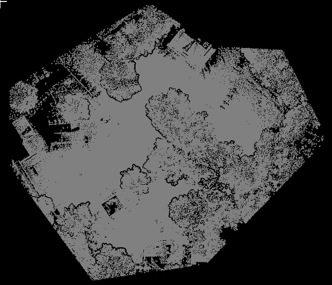
In our case, after noise removal, we got the result shown in Figure 24.
Figure 24. Noise removal result.
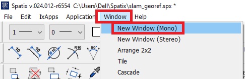
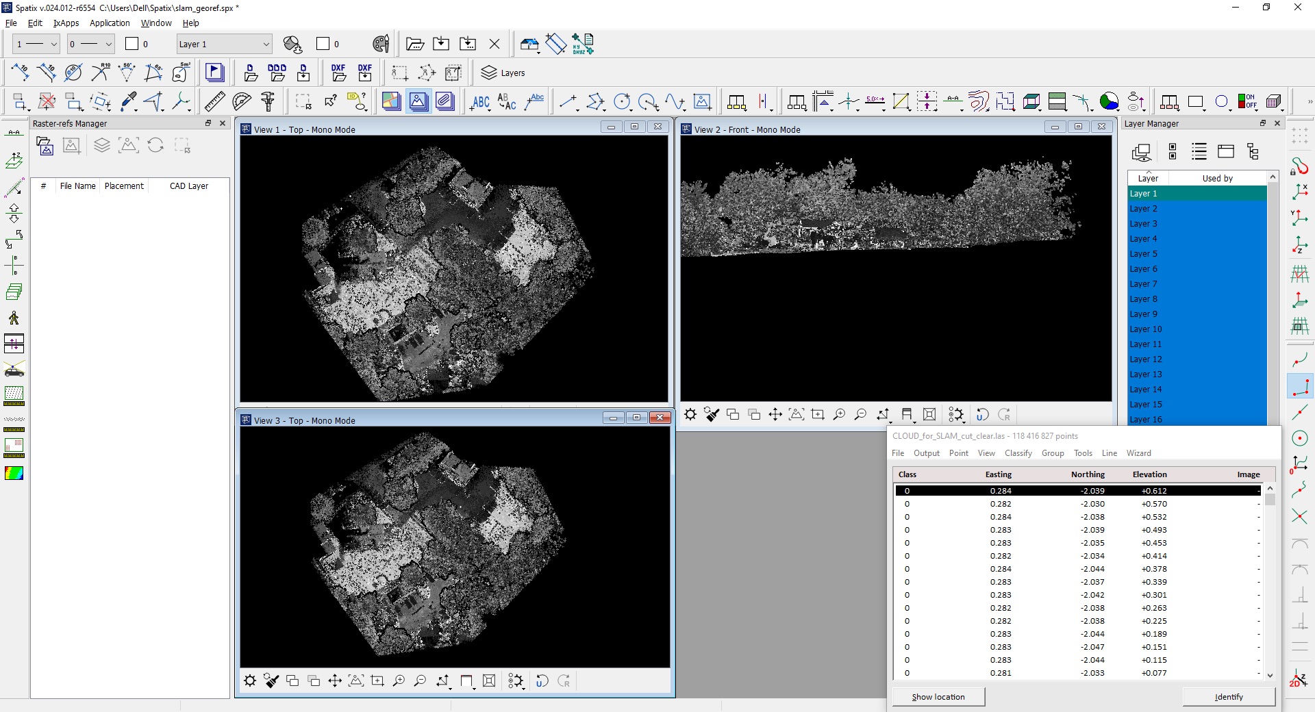
Now let’s examine the georeferencing procedure using control points. We will need an additional tool, which is available from the View Laser toolbar, Figure 25. Attach it on the left side of the main program window. Also, add a third view window. To do this, click on “Window” -> “New Window (Mono)” in the Spatix menu, Figure 26. We will need the third viewer to select targets in the point cloud. In addition, go to “View” -> “Display mode” and change the coloring of the point cloud in all three windows to “Intensity auto”. This will make it easier to find and recognize targets in the point cloud.
After the above-described steps, the main program window looks as shown in Figure 27.
Figure 25. "View Laser" Toolbox.
Figure 26. Adding a new view window.
Figure 27. The main program window after adding the third view window and fixing the toolbar on the left side.
After that, we can start georeferencing the SLAM point cloud.
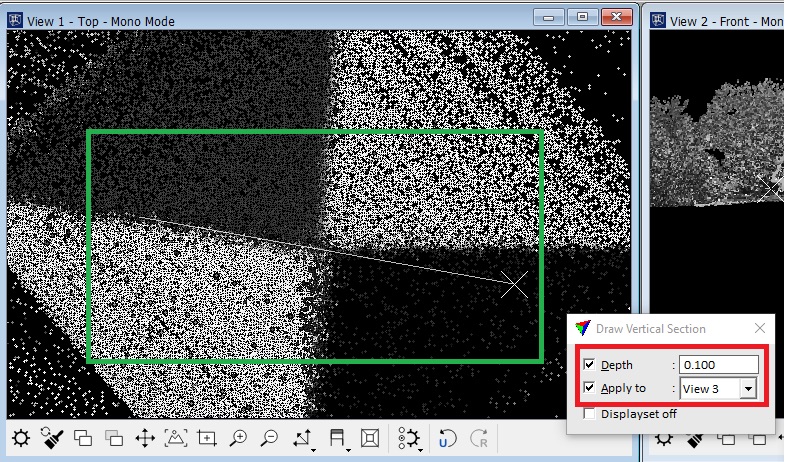
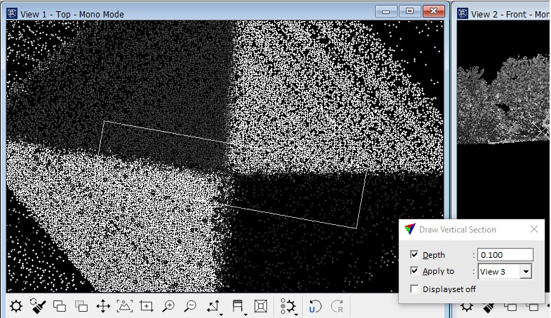
Select the profile view tool on the “View Laser” panel. Click on the “Draw Vertical Section” icon, and the window shown in Figure 28 will open. Here we set the depth of the point cloud and apply it to the 3rd view window. Now you should draw a line along the reference point. In this case, it is a line through the center of the target. Click on one end of the target and draw a line to the other end so that the center of the target coincides with the line. Click on the other end. A rectangle will appear, as shown in Figure 29.
Figure 28. Drawing a cut line through the center of the target.
Figure 29. The rectangle along which the point cloud will be cut.
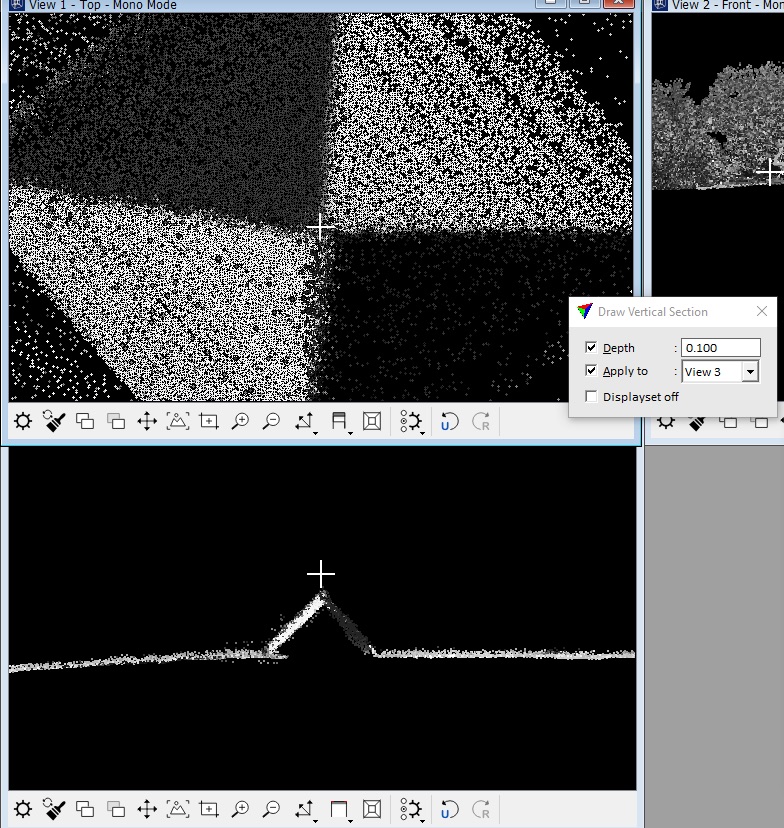
As a result, the third view window will show the point cloud cut as shown in Figure 30.
Figure 30. Section of the point cloud in the third view window.
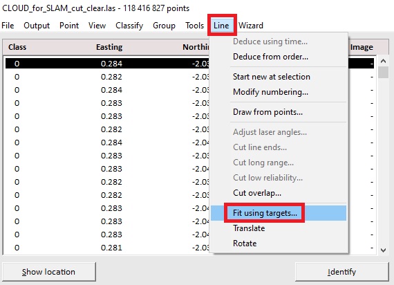
Now let’s add a control point. Click on “Line” -> “Fit using targets…” as shown in Figure 31.
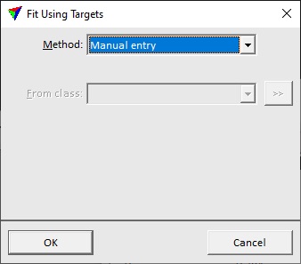
This will open a window where you can select the type of georeferencing data, as shown in Figure 32. We will use “Manual entry”. Click “OK”.
Figure 31. Data georeferencing menu.
Figure 32. Selecting the type of georeferencing.
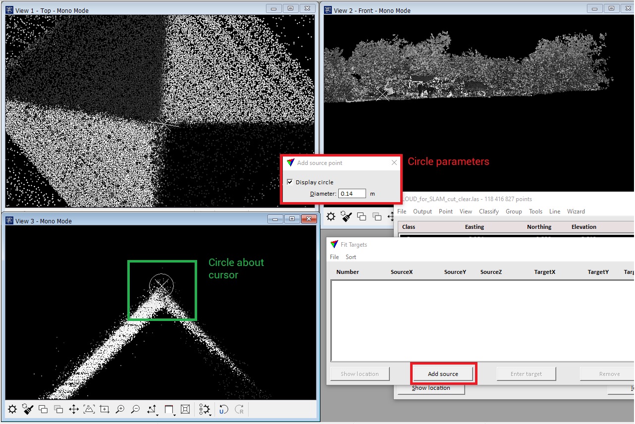
In the “Fit Targets” window, click on “Add source”, as shown in Figure 33. A circle will appear around the cursor and a window will open where you can customize the circle radius and its display. We will leave these parameters unchanged. Now put the cursor on the top of our target and click on it. Our local point will appear in the “Fit Targets” window.
Look for the next target, make a cut, and add another point. Repeat the procedure for at least three points.
Figure 33. Adding point coordinates to the list of points for georeferencing.
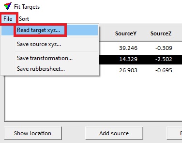
After selecting the points, click on “File” -> “Read target xyz…” as shown in Figure 34. A window will open with the path to the file with the target coordinates. After selecting the file, the list of points in the window will be updated with the target points as shown in Figure 35.
Figure 34. Menu for selecting a target point file.
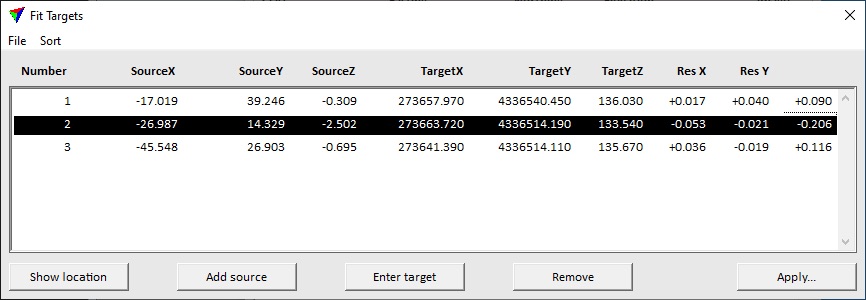
Figure 35. Updated list of source and target points.
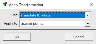
Click “Apply”, then select the transformation type in the window and apply it to the loaded points, as shown in Figure 36. A window opens with the choice of resolution. Click on “OK”.
Figure 36. Selecting the transformation type.
After the transformation was completed, the SLAM point cloud became geo-referenced, as shown in Figure 37.
Figure 37. Point cloud with new coordinates.
Now we will merge the resulting cloud with the cloud obtained by airborne scanning. To do this you need to:
Click “File” -> “Read points” and select the georeferenced Aerial point cloud. Of course, it should first be cleaned of noise in the same way we demonstrated for SLAM data.
Now we can evaluate the accuracy of our georeferencing using a report.
The control point report tool will create a report about the elevation difference between laser point clouds and ground control points, which can be used to check the elevation accuracy of laser point clouds and improve the height accuracy of laser point clouds using calculated adjusted values.
To create a report, you need to:
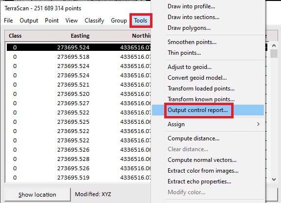
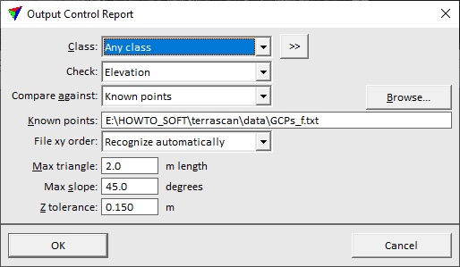
Click on the menu “Tools” -> “Output control report…” as shown in Figure 38. A window will open in which you have to choose the path to the file with control points and the threshold values above which the point will be considered as unlikelier, as shown in Figure 39.
Figure 38. "Output control report" tool.
Figure 39. "Output control report" parameters.
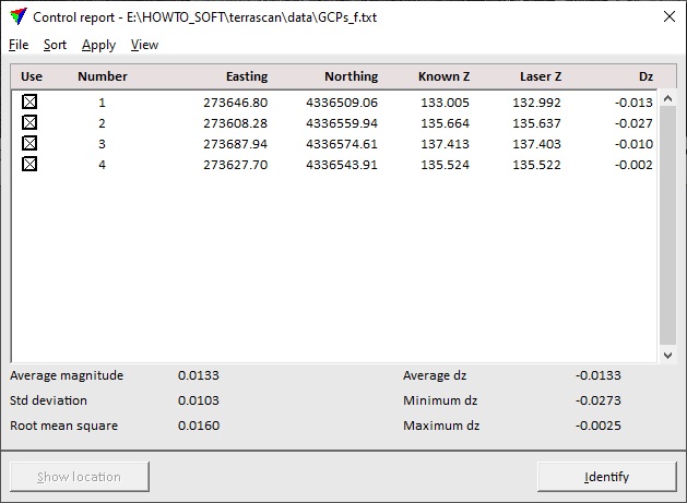
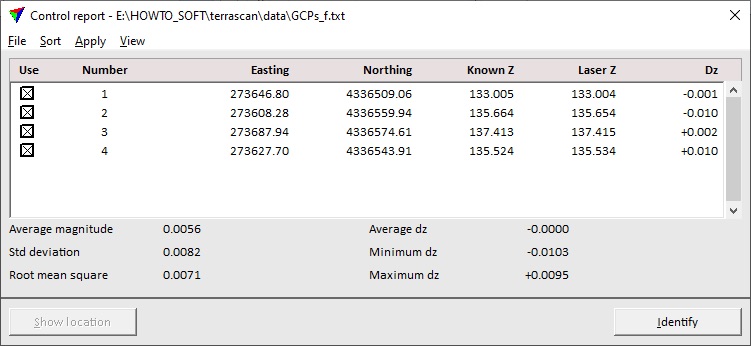
Choose the file path, the class, and the type of checkpoint. In this case, we will check the height deviation. Click on “OK”. After the calculation, the window shown in Figure 40 will open, displaying the list of checkpoints and the accuracy results. As you can see, we have obtained a very high georeferencing accuracy. The average value of “dz” is less than 2 cm.
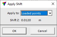
To immediately apply the calculated shift to the point cloud, click “Apply” -> “Elevation shift…” in the menu. The window shown in Figure 41 will open, where you can select which points the shift will be applied to. We will apply the shift to all loaded points, so click “OK”.
Figure 40. The result of the accuracy calculation.
Figure 41. "Apply Shift" parameters.
After this, the shift will be applied to the entire point cloud, and the values in the “Control report” window will change taking into account the shift. The result of the operation is shown in Figure 42.
Figure 42. As a result of the height correction, the average error value = 0
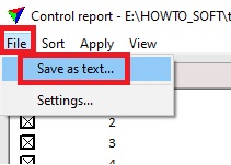
The obtained report can be saved as a text file. To do this, click in the menu “File” -> “Save as text…”, Figure 43. Then specify the name of the file and the path where you want to save it.
Figure 43. Saving the report to a text file.
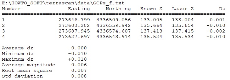
The report will contain information about the control points and the results of the calculated accuracy, as shown in Figure 44. The saved report can be easily distributed to clients.
Figure 44. Z-Accuracy report.
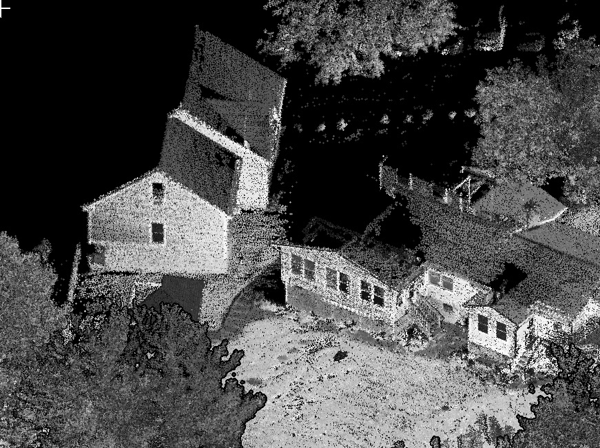
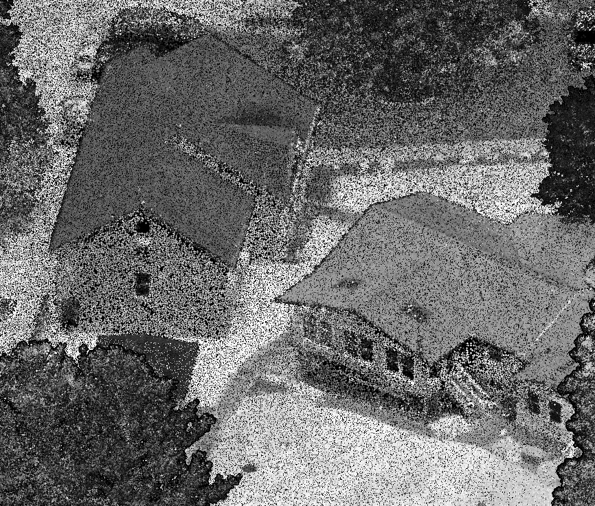
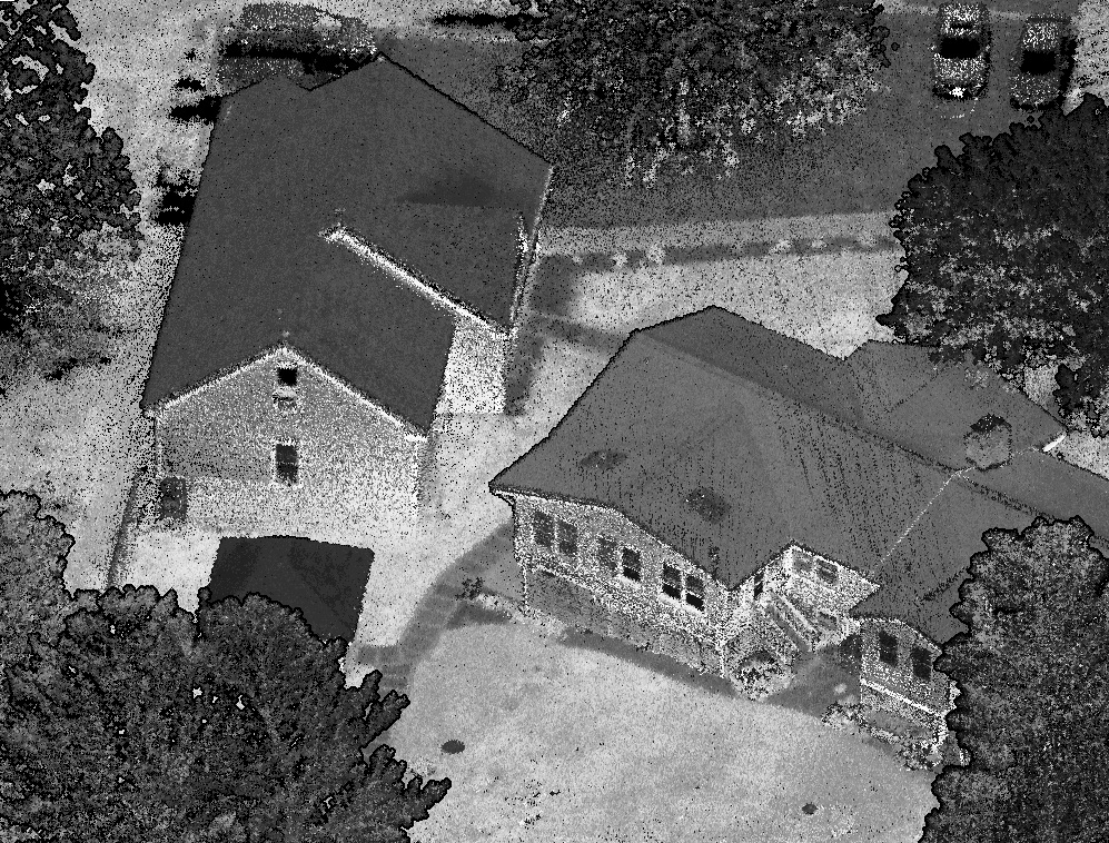
Let’s take a closer look at the obtained result, which is shown in Figure 45-47.
Figure 45. Slam Point Cloud (raw data).
Figure 46. Aerial Point Cloud (raw data).
Figure 47. SLAM + Aerial Point Cloud.
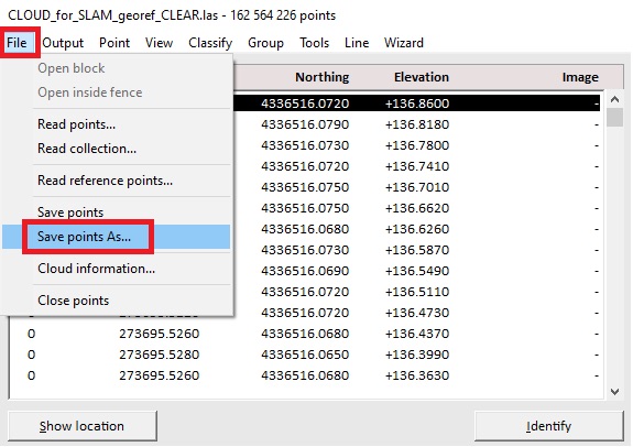
To save the processed cloud, follow these steps:
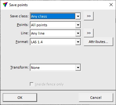
Click “File” -> “Save points As…”, Figure 48. After that, a window will open, Figure 49, where you can customize the file parameters. After customization click “OK”. A standard save window will open, where you specify the name of the file and the path where you want to save it.