An orthomosaic is a commonly implemented geospatial deliverable created using images. This guide will show how to generate orthomosaics from images captured by RESEPI in Agisoft Metashape Proffesional by Agisoft. We will also cover key aspects to pay attention to.
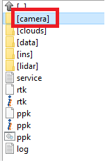
After processing LiDAR data in PCMasterPro, the project folder will look as shown in Figure 1.
Figure 1. Folder structure after processing in PCMasterPro.
We are particularly interested in the folder named “Camera,” which contains all the photos obtained during data collection. It is also important to have a file with Ground Control Points (GCPs) for georeferencing. The more accurately the GCPs are measured, the higher the accuracy of the orthomosaic georeferencing.
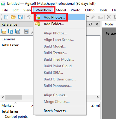
To generate an orthomosaic, you need to create a project and import images. This can be done by importing the photos directly or specifying the path to the folder containing them.
To do this, click the “Workflow” -> “Add Photos…”, as shown in Figure 2. A window will open where you need to select the path to the images and choose the photos you want to process. In our case, we import all photos from the “Camera” folder.
Figure 2. Importing images menu.
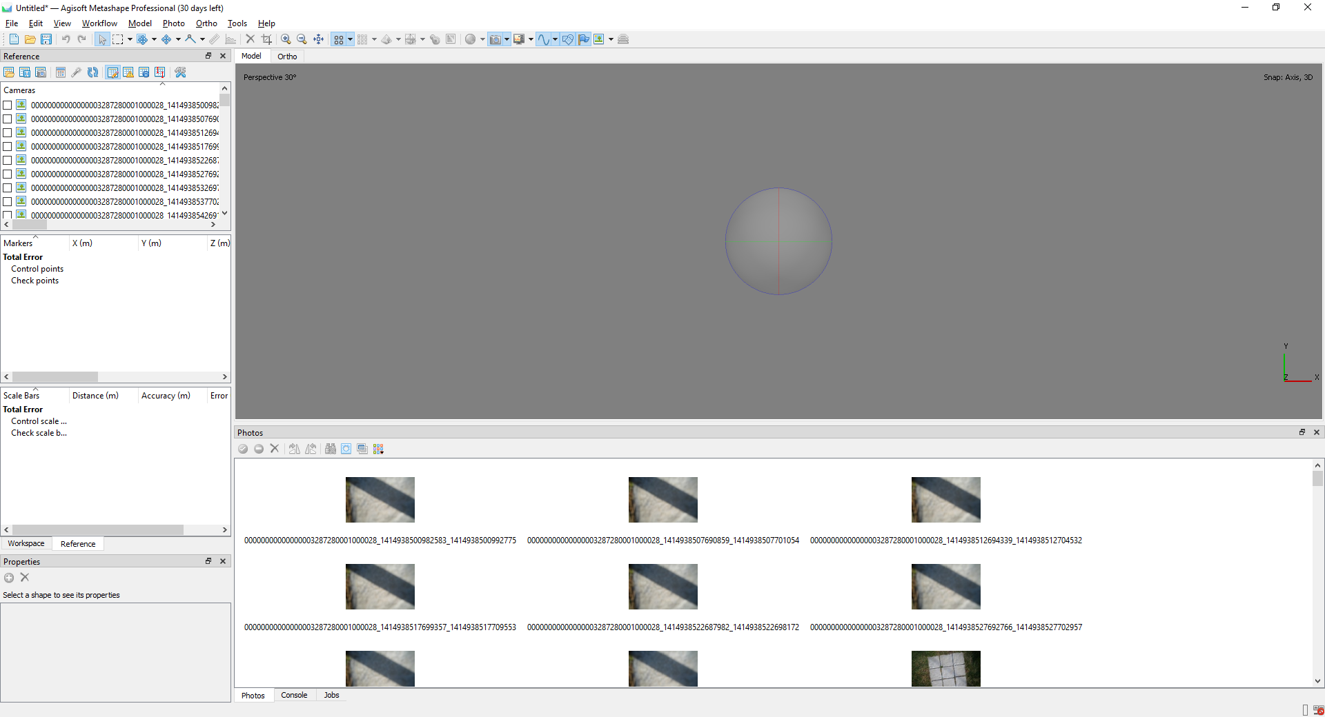
After importing the images, the main window of the program will look as shown in Figure 3.
Figure 3. Main program window after importing images.
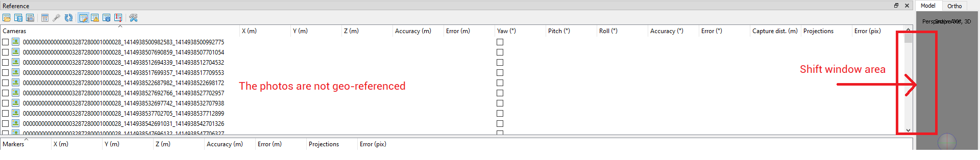
If we shift the window area to the right, we will see that our images do not have georeferencing data since EXIF metadata lacks coordinates, as shown in Figure 4. Therefore, we will manually georeference the images using Ground Control Points (GCPs).
Figure 4. Missing coordinate and orientation data fields.
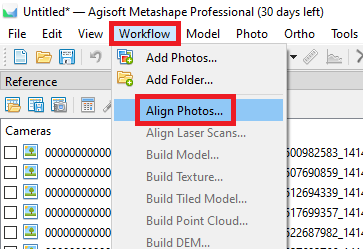
After loading the images into the program, they should be aligned. To do this, click “Workflow” -> “Align Photos…” as shown in Figure 5.
Figure 5. Aligning photos menu.
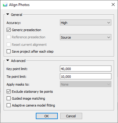
A window will open, as shown in Figure 6, where alignment parameters can be configured. We use the same parameters as in the figure. Click “OK” and wait for the alignment process to complete.
Figure 6. Photo alignment parameters.
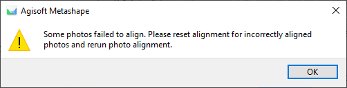
• After alignment, a warning window may appear, as shown in Figure 7, indicating that some photos could not be aligned. Simply click “OK”.
Figure 7. Informational warning.
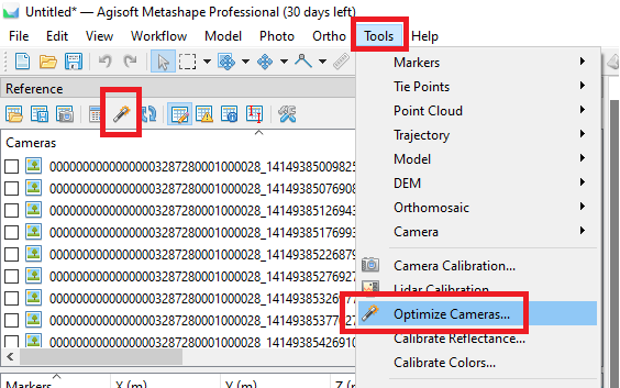
The next step is to optimize alignment. Click the “Optimize Alignment” icon in the “Reference” tab or use “Tools” -> “Optimize Cameras…” as shown in Figure 8.
Figure 8. Optimization menu.
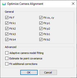
A window with optimization parameters will open, as shown in Figure 9. We activated all 10 parameters.
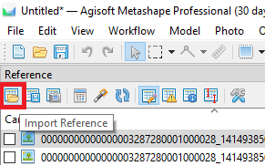
Click the “Import Reference” icon, as shown in Figure 10.
Figure 10. Importing control points.
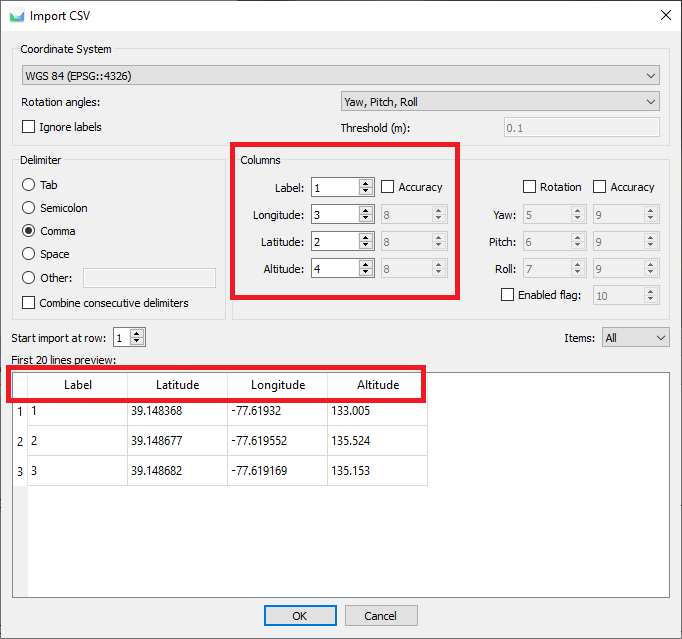
A window will open where you can select the GCP file. After selecting the file, another window will appear, as shown in Figure 11. Here, it is crucial to set the correct column order so that the program reads the data correctly. Click.
Figure 11. Import parameters for GCP file.
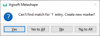
Since the images do not have georeferencing, the program cannot automatically place markers. A window will appear, as shown in Figure 12. Click “Yes to All” to manually place them.
Figure 12. Confirmation for creating new markers.
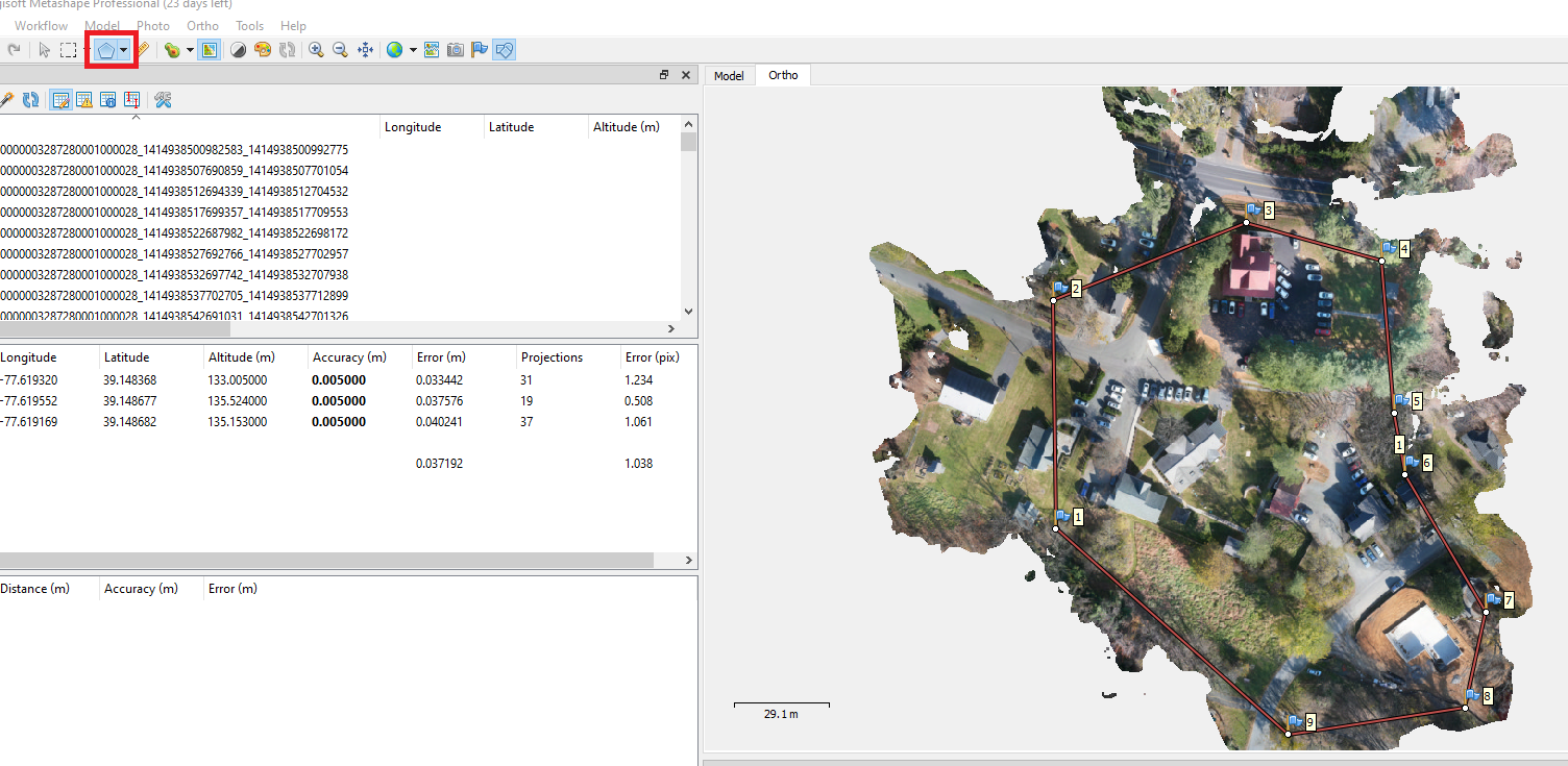
The Ground Control Points will then appear in the list, as shown in Figure 13. Next, we will filter and disable unnecessary images, such as those captured at takeoff and landing.
Figure 13. Main program window after adding control points.
To disable unnecessary images, select them and click “Disable Images” in the “Photos” panel. This ensures they are not used in processing.
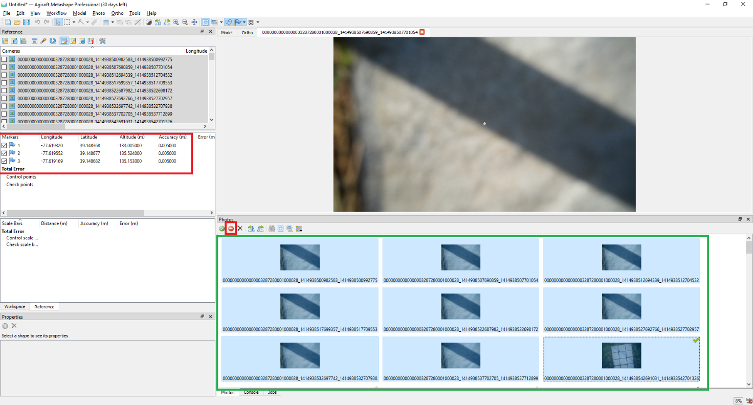
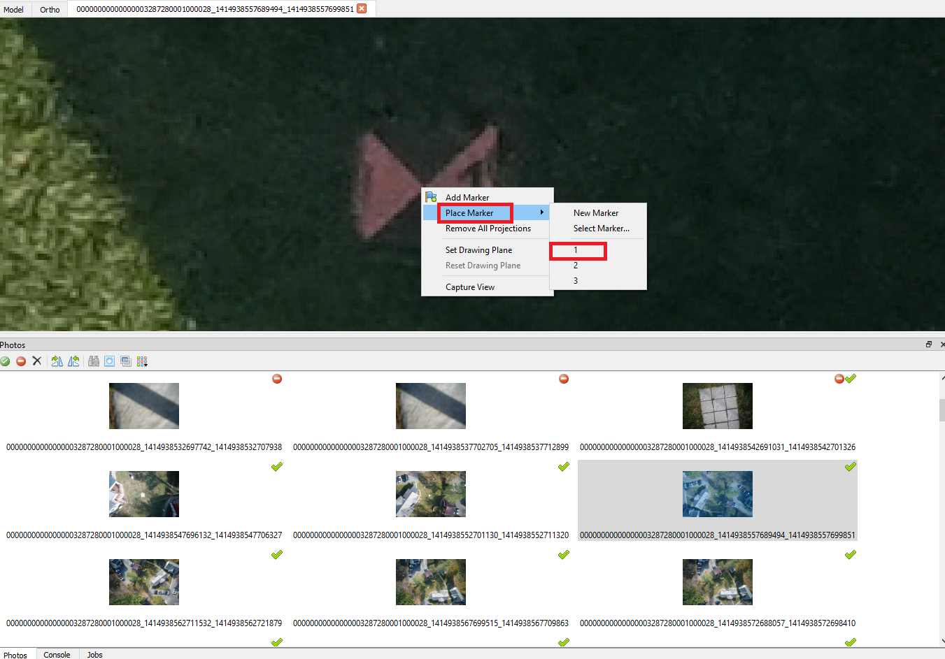
Next, find an image with a visible target, double-click it, and place a marker using “Place Marker” from the right-click menu, aligning it with the center of the target, as shown in Figure 14.
Repeat this for another image with the same target.
Figure 14. Placing a marker on a target.
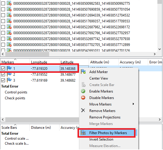
The program will then automatically detect the corresponding images. To make further tagging easier, right-click the marker in the control point list and select “Filter Photos by Markers” as shown in Figure 15.
Figure 15. Filtering images by marker.
Adjust markers manually if needed. Repeat this process for all control points.
Repeat the steps for the rest of the reference points. You can also switch between photos using the “Reference” -> “Cameras” panel by double-clicking on a photo.
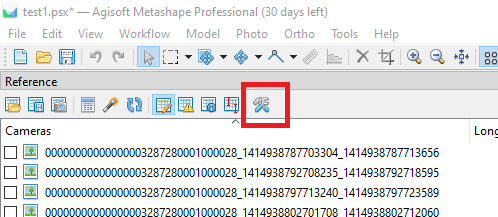
Click “Reference Settings” in the “Reference” panel, as shown in Figure 16.
Figure 16. Reference Settings.
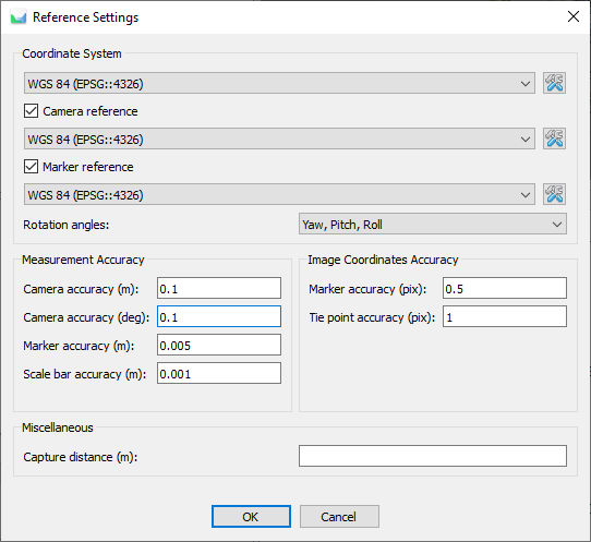
In the settings window (Figure 17), configure accuracy and coordinate system parameters.
Figure 17. Reference settings window.
After that, we can proceed to constructing the point cloud.
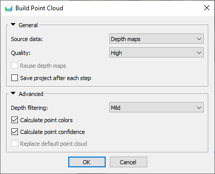
Click “Workflow” -> “Build Point Cloud…” as shown in Figure 18. Select the parameters and click “OK”. The process may take some time depending on your PC’s processing power.
Figure 18. Point cloud generation parameters.
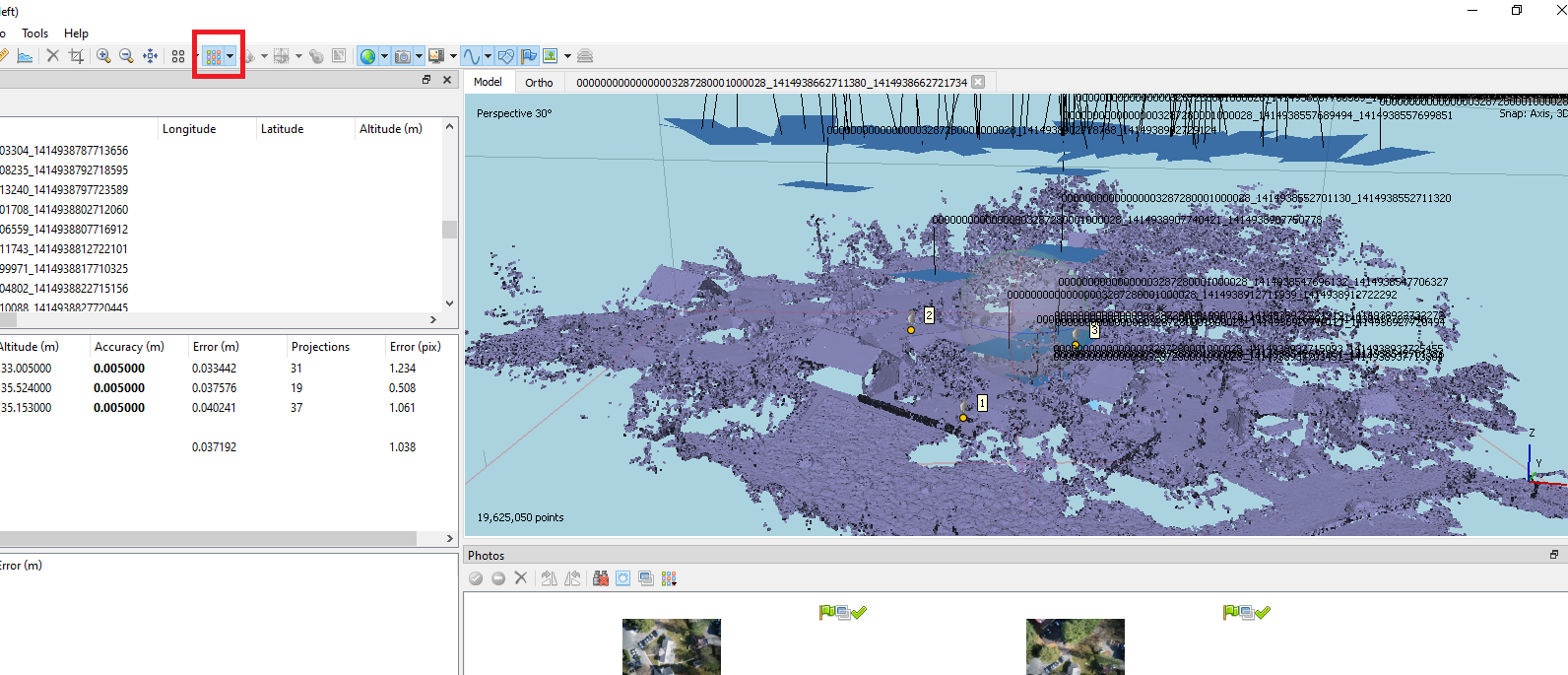
Once the process is complete, click the “Point Cloud” icon to display the generated point cloud, as shown in Figure 19.
The next step is to build the model from which the orthomosaic will be generated.
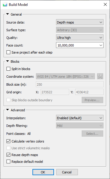
Click “Workflow” -> “Build Orthomosaic…” as shown in Figure 20. Configure parameters and click “OK” to start the process.
Figure 20. Model generation parameters.
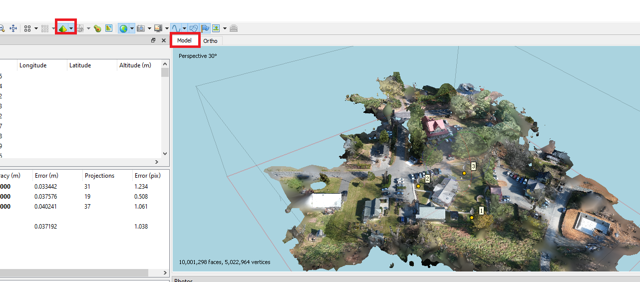
Once the process is complete, switch to the “Model” tab and click on the “Model” icon as shown in Figure 21. A three-dimensional surface model will be displayed in the viewing area.
Figure 21. Displaying the model.
Next, we proceed to the building of the orthomosaic.
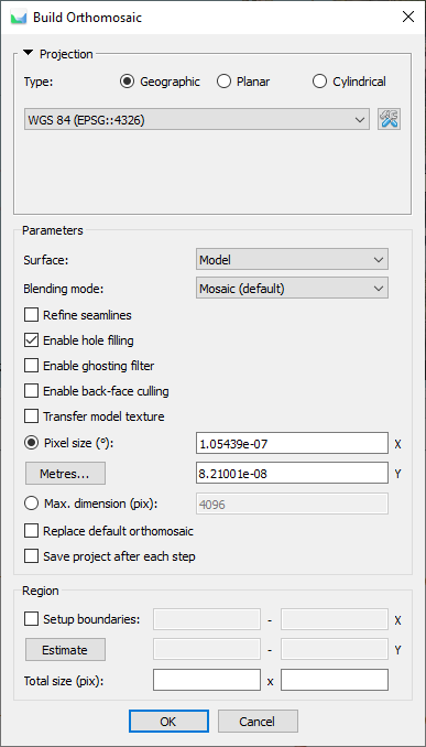
To do this, click on the menu “Workflow” -> “Build Orthomosaic…”. The window shown in Figure 22 will open. Select the parameters and click “OK”. The process of building Orthomosaic will start.
Figure 22. Orthomosaic generation parameters.
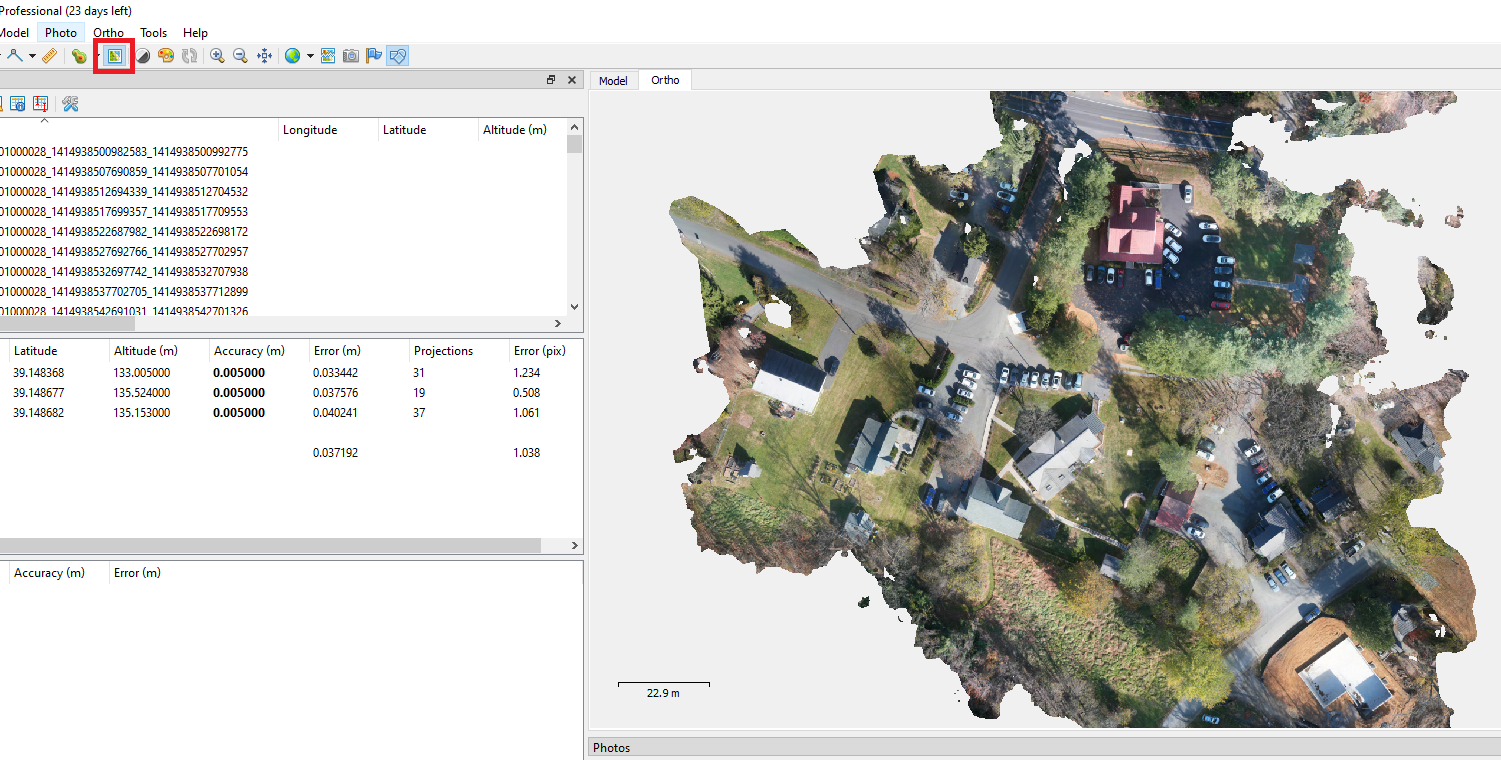
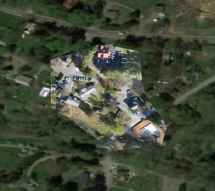
After processing, click the “Orthomosaic” icon to display the final result, as shown in Figure 23.
Figure 23. Displaying the orthomosaic.
Generating a Report
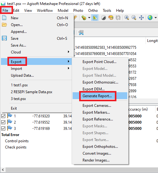
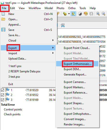
To assess orthomosaic quality, generate a report via “File” -> “Export” -> “Generate Report…” as shown in Figure 24.
Figure 24. Report generation menu.
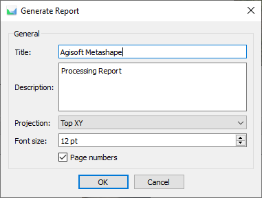
In the settings window (Figure 25), configure report parameters and click “OK.” Save the report as a .pdf file.
Figure 25. Report generation settings.
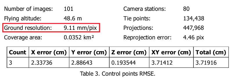
Now we can see the results of georeferencing accuracy as well as Ground resolution as shown in Figure 26. As you can see, we got a great result, GSD is less than 1 cm and RMS of georeferencing is less than 1 cm.