Contour lines, the Digital Elevation Model (DEM), Digital Terrain Model (DTM) and the Digital Surface Model (DSM) are commonly used geospatial deliverables created using point clouds. This guide will show how to retrieve these models from a point cloud from RESEPI in CloudCompare. We will also look at how to generate reports and highlight the key aspects to consider.
Any activity with point clouds begins with the import of data. In CloudCompare, this can be done in several ways:
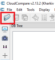
Use the Quick Access menu in the upper-left corner, as shown in Figure 1.
Click on the “File” button, and then click on “Open”.
This will open a window where you need to specify the path to the .las (.laz) file.
Figure 1. Import data.
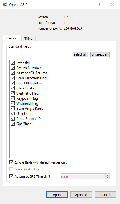
A window with import parameters will appear, as shown in Figure 2. Just click “Apply”.
Figure 2. Import Parameters.
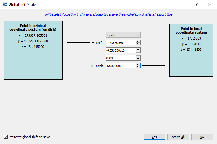
A window with scaling settings will appear, as shown in Figure 3. Click “Yes”.
Figure 3. Scaling Parameters.
As a result, our point cloud will be displayed in the main window, as shown in Figure 4.
Select the cloud in the project tree and set “Intensity” in the coloring parameters. Set the color scale to “Blue>Green>Yellow>Red”. Use the sliders with a triangle to change the coloring range.
The next step is to prepare the point cloud for DSM, DEM, and Contours. To do this, we’ll use the crop tool to remove unrequired points and thin out the clouds. This step will also speed up data processing.
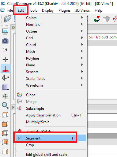
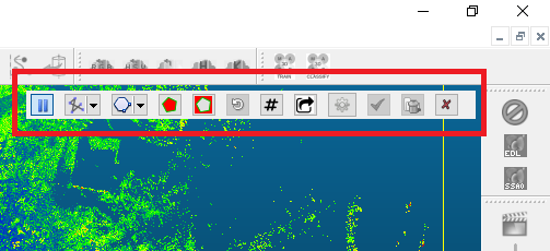
To remove the extra points, click on the “Edit” -> “Segment”, as shown in Figure 5.
Figure 5. "Segment" tool menu.
The panel shown in Figure 6 will appear. Here we select the polygon selection. After selecting the desired area of the point cloud, click on “Segment In (I)” to leave the selected area for further processing. To delete the selected area, click “Segment Out (O)”.
Figure 6. "Segment" tool panel.
After clearing the point cloud of unnecessary points, click on the green checkmark in the “Segment” toolbar.
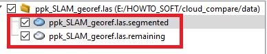
As a result, the original point cloud will be divided into two parts defined by the “Segment” tool. The project tree panel will display two files, one of which is the section of the point cloud that we have selected for further processing, and the second file contains all the remaining points, as shown in Figure 7.
Figure 7. View of the project tree panel after using the "Segment" tool.
If for some reason you accidentally marked unnecessary areas of the point cloud, or did not delete unnecessary areas, then everything can be fixed by “gluing” the separated parts. To do this, click on the “Edit” -> “Merge” menu.
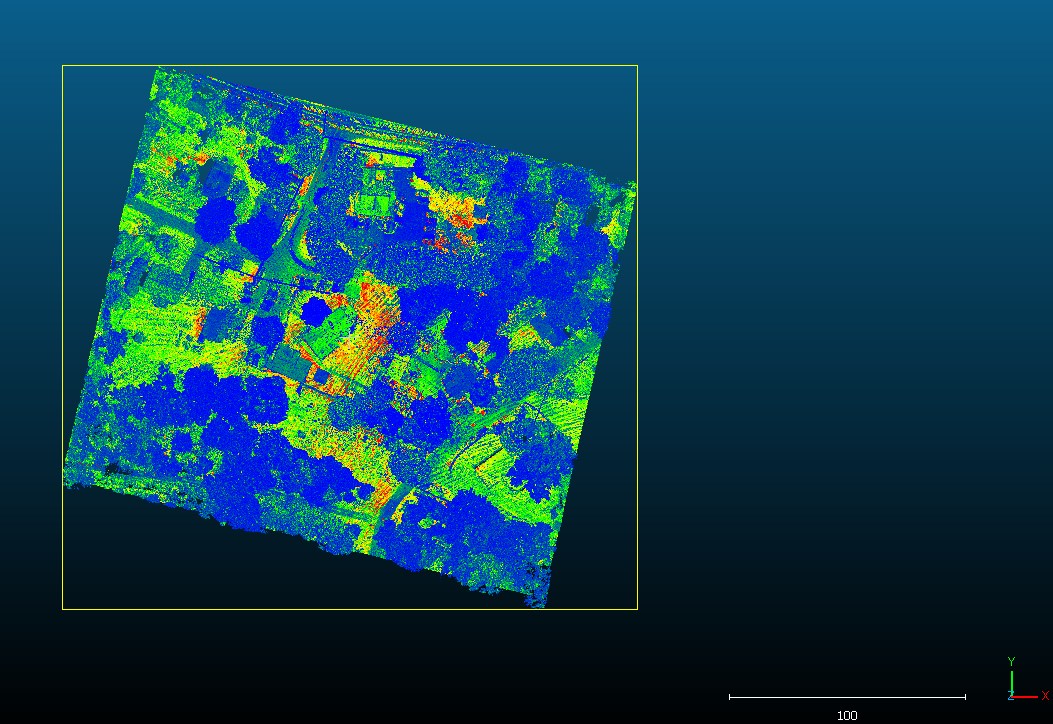
We selected the area of interest to us, which is shown in Figure 8.
Figure 8. Point cloud after cropping.
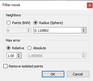
Next, we filter the cloud using “Noise Filter”. To do this, click on “Tools” -> “Clean” -> “Noise Filter”. A window with filtering parameters will open, which is shown in Figure 9. Click “OK” and wait for the filtering process to complete.
Figure 9. Filtering parameters.
After filtering, a file with the word “clean” at the end of the file name will be displayed in the project tree panel. This is the filtered file that we will use to generate DEM and DSM.
We recommend saving the resulting file. This can be done by selecting it in the project tree panel and then clicking “File” -> “Save”. There are many popular formats available for saving.
Point Cloud to Digital Elevation Model and Digital Surface Model#
To generate DEM, we will need to separate the ground points. To do this, we will use the CSF plugin, which is available from the “Plugins” -> “CSF Filter” menu.
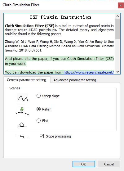
The window shown in Figure 10 contains the filtering parameters for separating ground points from all other points.
Figure 10. "CSF Filter" parameters.
Select the surface type in the “General parameter setting” tab and set the surface modeling parameters in the “Advanced parameter setting” tab. Click “OK”.
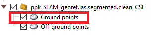
After separating the ground points, the files into which the point cloud was divided after applying CSF will appear in the project tree panel, as shown in Figure 11.
Figure 11. Ground points and Off-ground points.
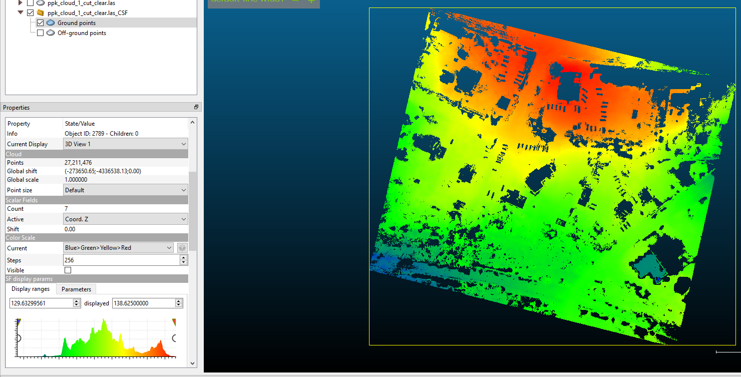
The next step is to set the color of the future DEM raster. To do this, select “Ground Points” and click in the menu “Edit” -> “Scalar fields” -> “Export coordinate(s) to SF(s)” and select the “Z” coordinate. This way we can change the coloring of the points by height, not by intensity, as shown in Figure 12. Use the sliders to set the scale range.
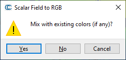
In addition, we transform our scalar field to RGB. Click “Edit -> Scalar fields -> Convert to RGB”. The window shown in Figure 13 will open. Click “No”.
Figure 12. After creating a scalar field with the "Z" coordinate, you can color the points by height.
Figure 13. Scalar field to RGB.
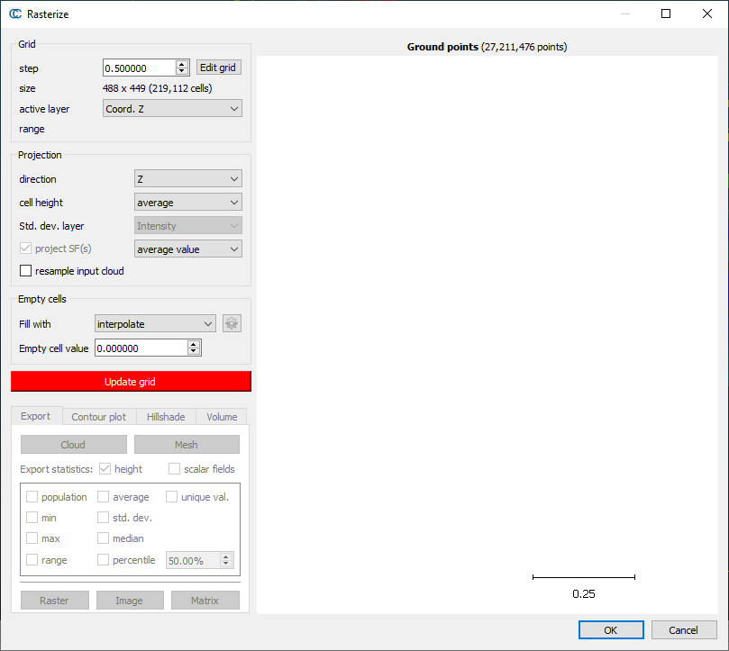
To generate DEM, select the “Ground Points” file and click on “Tools” -> “Projection” -> “Rasterize (and contour plot)”. The window shown in Figure 14 will open.
Figure 14. "Rasterize" parameters.
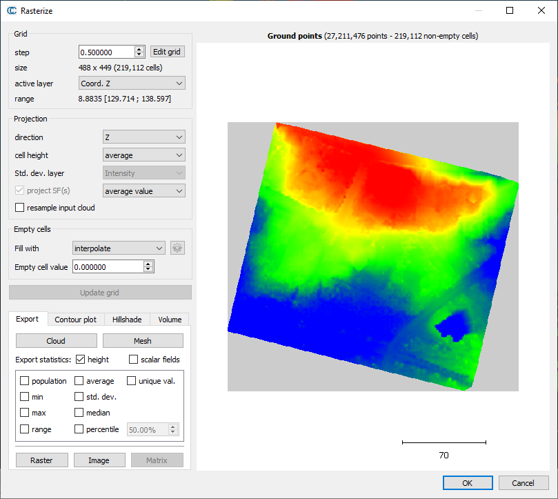
Set the parameters, click on “Update grid”, after which a raster image will be displayed in the viewing window, as shown in Figure 15.
Figure 15. Rasterization result.
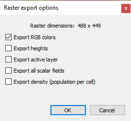
To export the obtained result to a file, click on “Raster”. A window with a choice of export parameters will open, which is shown in Figure 16. Click “OK”. A standard window will open, in which you specify the file name and the path where you want to save the file.
Figure 16. Export parameters.
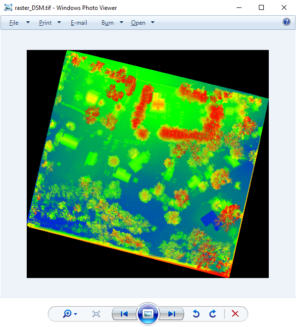
To generate DSM, repeat the above procedure using the prepared point cloud. We will not repeat all the steps again, but will only show the results, which are shown in Figure 17 and Figure 18.
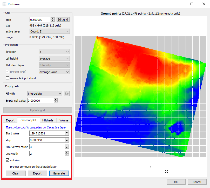
In the “Rasterize” window, go to the “Contour plot” tab and set the parameters as shown in Figure 19.
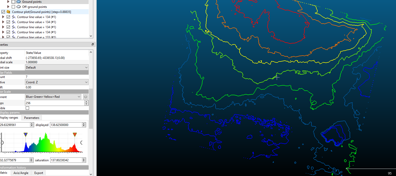
Click “Generate”, after which the contours will be displayed in the preview window. By clicking on “Export”, we export the contours to the “DB tree” (Figure 20). After that, they can be saved via the menu “File” -> “Save”.