Contour lines, the Digital Elevation Model (DEM), and the Digital Surface Model (DSM) are commonly used geospatial deliverables created using point clouds. This guide will show how to retrieve these models from a point cloud from RESEPI in Lidar 360 by Global Mapper Pro by Blue Marble Geographics. We will also look at how to generate reports and highlight the key aspects to consider.
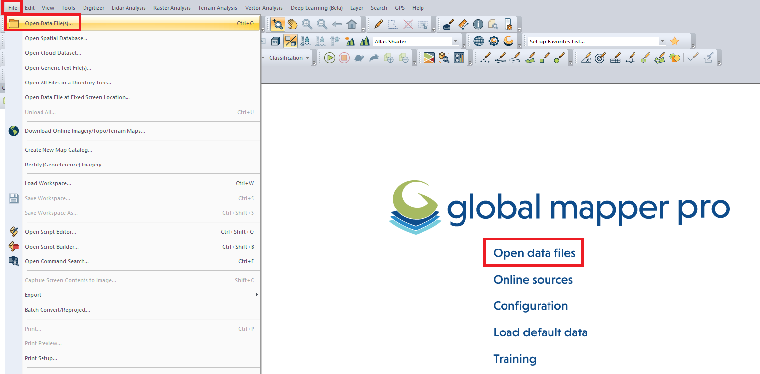
Any work with point clouds begins with data import. In Global Mapper Pro, this can be done via the menu “File” -> “Open Data File(s)” or by clicking “Open Data Files” on the program’s start page, as shown in Figure 1. A dialogue box will pop up to specify the path to the .las (.laz) file.
Figure 1. “Add Data” workflow.
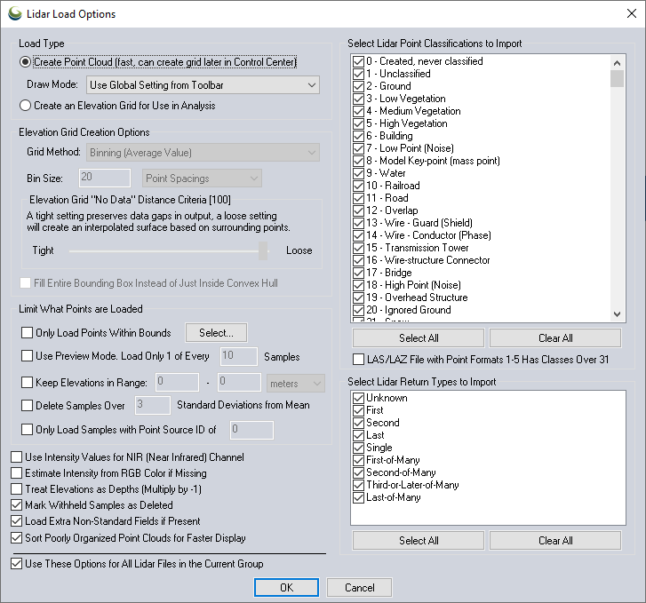
A window with import settings will open, as shown in Figure 2. Leave the default settings unchanged and click “OK.” The import process will begin, after which the main program window will appear, as shown in Figure 3.
Figure 2. Data Import Parameters.
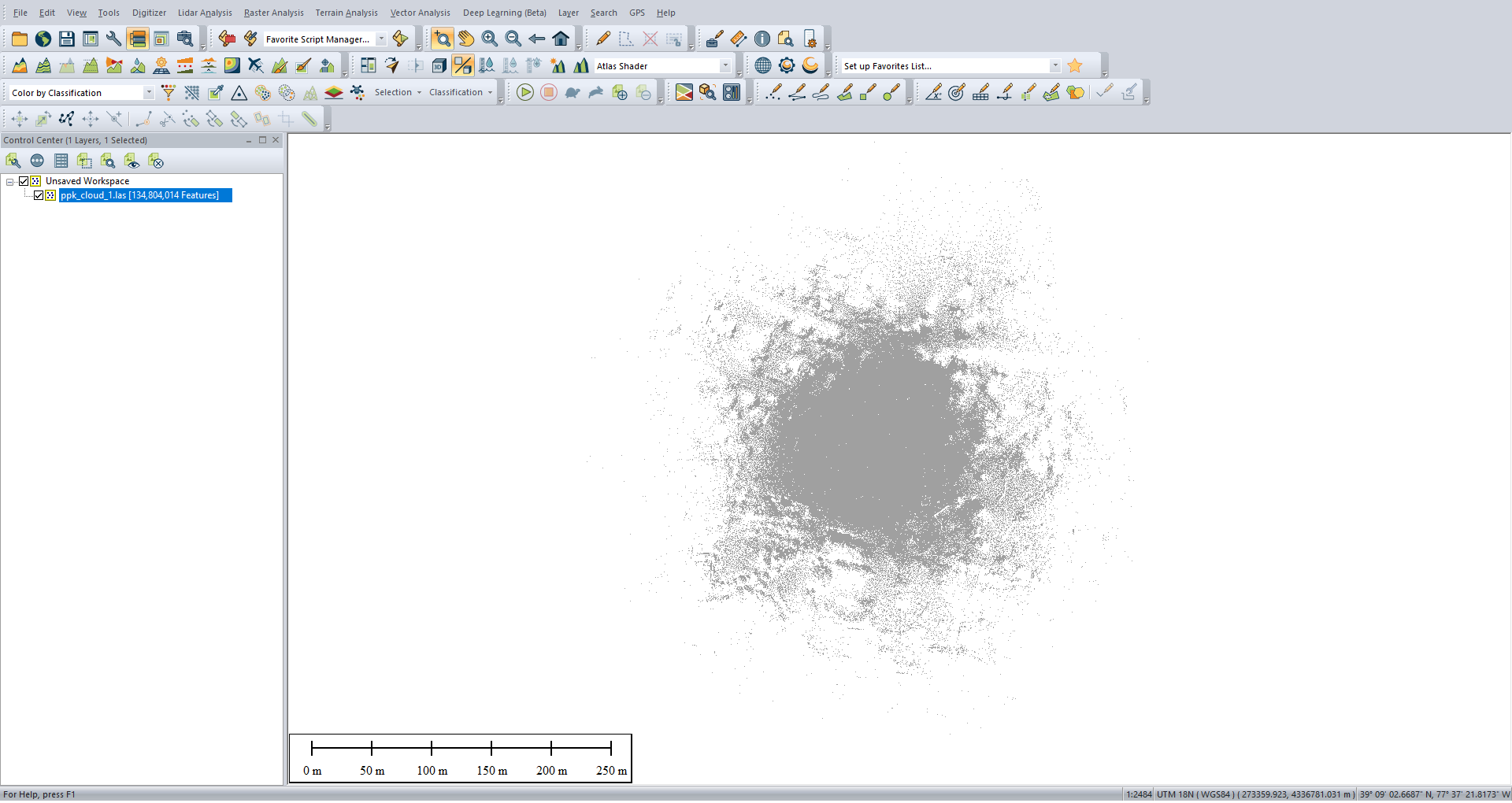
Figure 3. Main Program Window After Importing Data.
The next step is to prepare the point cloud for DSM, DEM, and Contours. To do this, we’ll use the crop tool to remove unrequired points and thin out the clouds. This step will also speed up data processing.
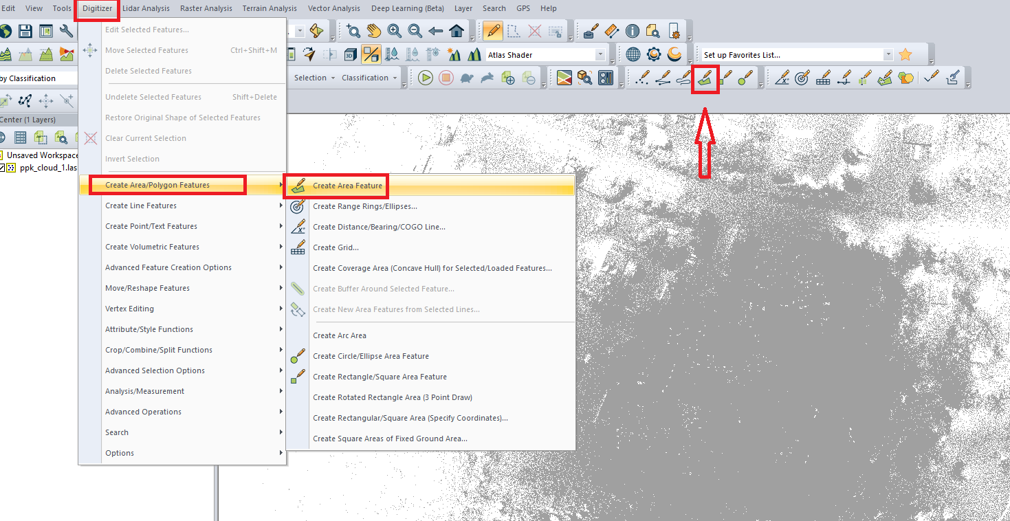
The first step will be to remove unnecessary points in the cloud. For this we will need the area creation tool, which is available from the menu “Digitizer” -> “Create Area/Polygon Features” -> “Create Area Feature”. You can also click on the icon in the toolbar, as shown in Figure 4.
Figure 4. Area creation tool.
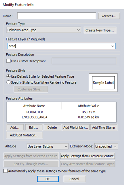
Select the tool and create an area in the desired area of the point cloud by clicking LMB (left mouse button) to fix the boundary lines. After creating the area, click RMB (right mouse button) to save the result. The window shown in Figure 5 will open. In this case, we will only assign a name to the area in the “Feature Layer” field, because this is a mandatory parameter. Click “OK”.
Figure 5. Area creation parameters.
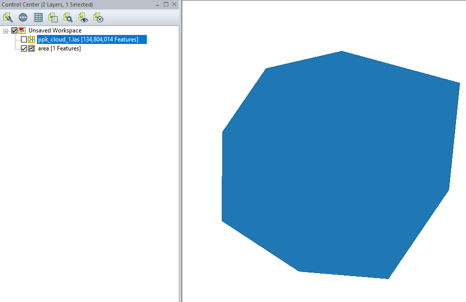
By unchecking the box next to the point cloud file, we hide it from the viewing window, thereby seeing the shape of our selected area to which we need to add points from the point cloud (Figure 6).
Figure 6. Shape of the selected area.
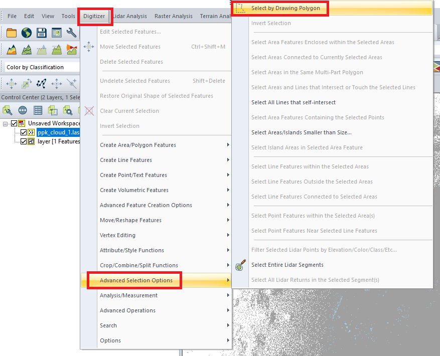
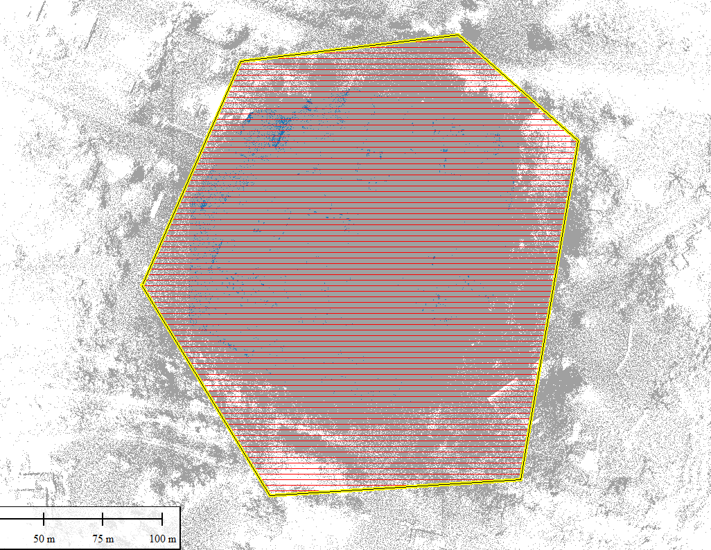
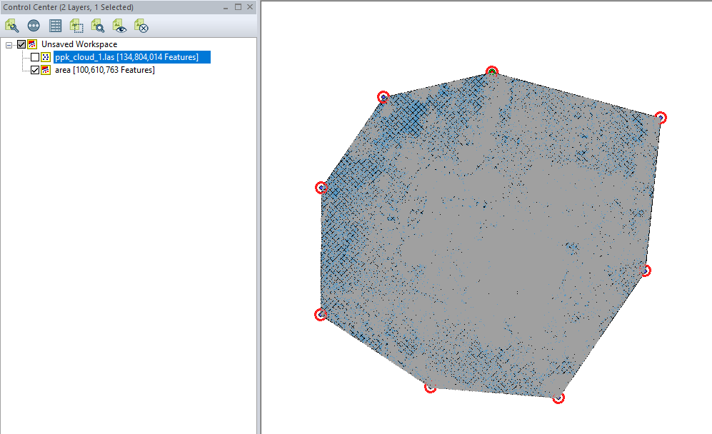
Next, we need to select the points from the cloud that we want to transfer to the area. We put a checkmark back to display the point cloud over the area and select the selection tool, which is available from the menu “Digitizer” -> “Advanced Selection Options” -> “Select by Drawing Polygon” (Figure 7). And we highlight the area, over-created “area” (Figure 8). The area will be highlighted in red.
Figure 7. Polygon selection tool.
Figure 8. The selected area over the created area.
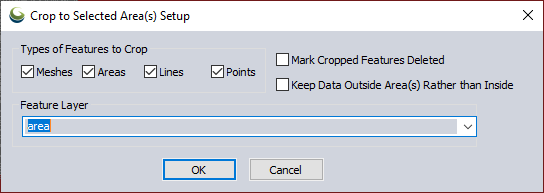
Immediately after this, click in the menu “Digitizer” -> “Crop/Combine/Split Functions” -> “Crop to Selected Areas…”. The window shown in Figure 9 will open. In the “Types of Features to Crop” field, you can choose which elements will be transferred to the new layer. We will leave the parameters unchanged and select the layer to which we want to assign the points in the “Feature Layer” field. Click “OK”.
Figure 9. Options for assigning data to a new layer.
As a result, we will get a ready area for further processing, as shown in Figure 10.
Figure 10. The area is ready for processing.
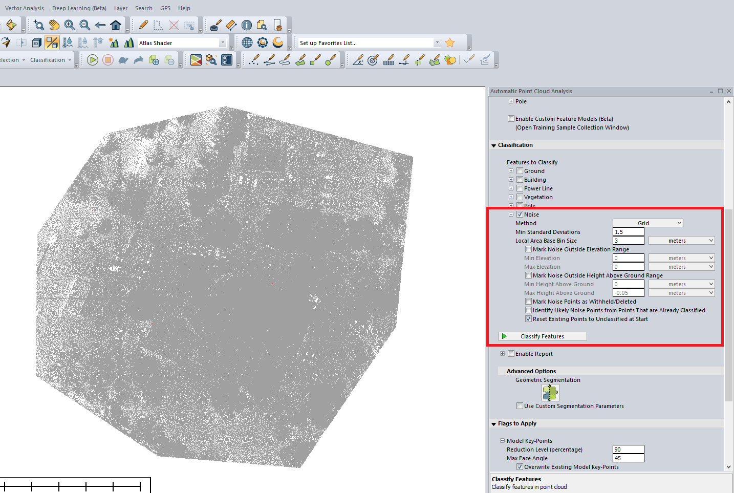
Next, we will remove noise. This can be done automatically, by classification, or manually. We will demonstrate both methods. The first method is available from the menu “Lidar Analysis” -> “Automatic Classification” -> “Noise Points…”. In the opened panel we set the parameters and click on “Classify Features” (Figure 11). It may be necessary to adjust the parameters and repeat the classification procedure to achieve a good result.
Figure 11. Noise classification parameters.
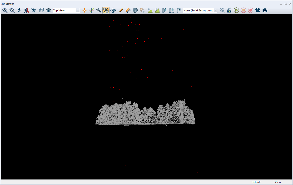
Once the classification is complete, you can quickly evaluate the result by clicking on “View” -> “3D View…”. A window will open in which you can freely rotate the point cloud and monitor the classification quality, as shown in Figure 12.
Figure 12. 3D viewing window.
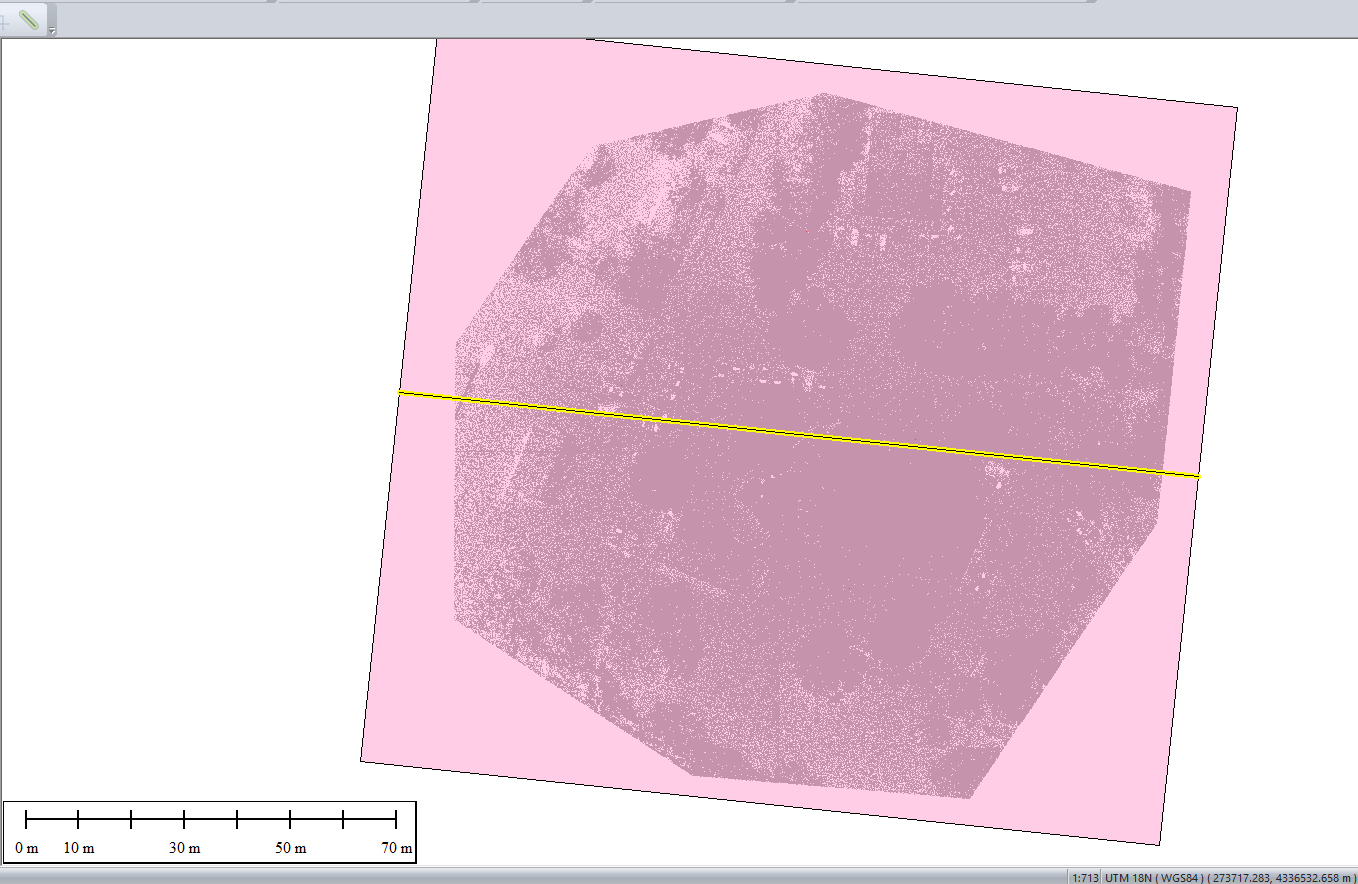
In our case, not all points were classified as noise, so we will use a manual classification method. To do this, we will make a cut of the entire point cloud along its entire length and width. Click in the menu “Tools” -> ” Path Profile/LOS” and draw a line along the entire length of the point cloud, as shown in Figure 13.
Figure 13. Point cloud cutting line.
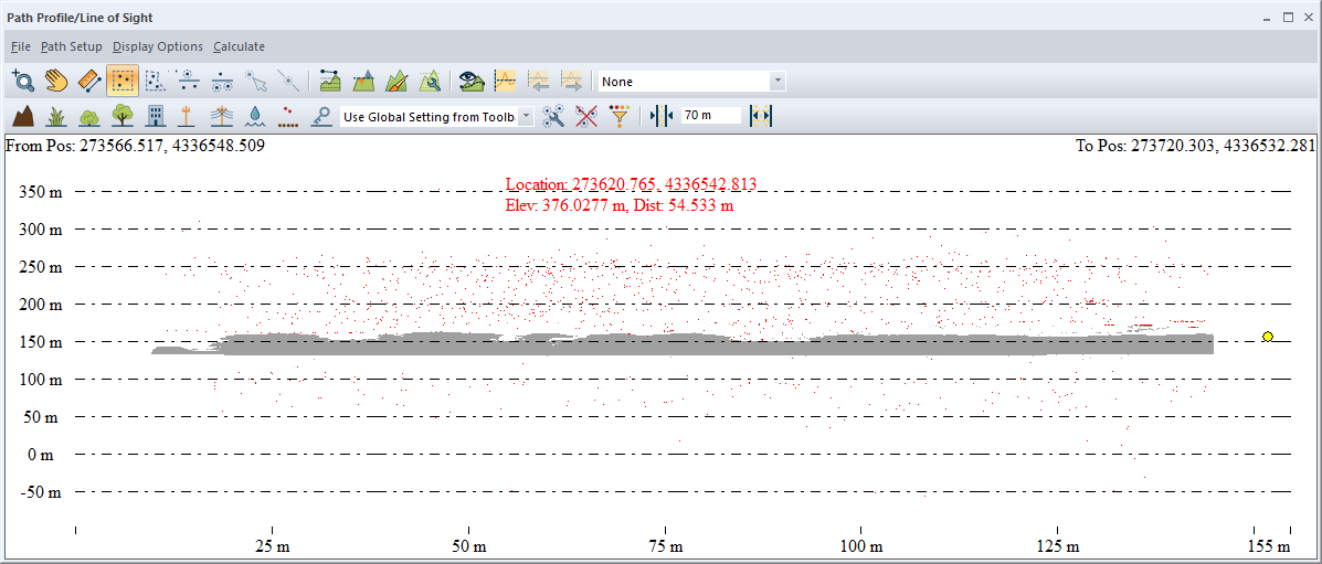
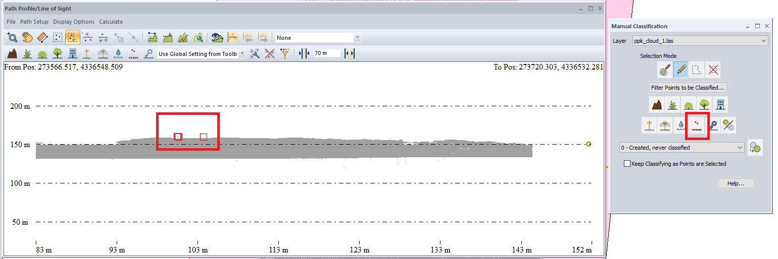
We have previously set the corridor width suitable for our point cloud. In the point cloud profile view window (Figure 14), this can be done by setting the width value in the corresponding field. As you can see, the noise at the bottom and top of the point cloud is marked in red; it remains to select those points that were not determined by automatic classification.
Figure 14. "Path Profile/Line of Sight" window.
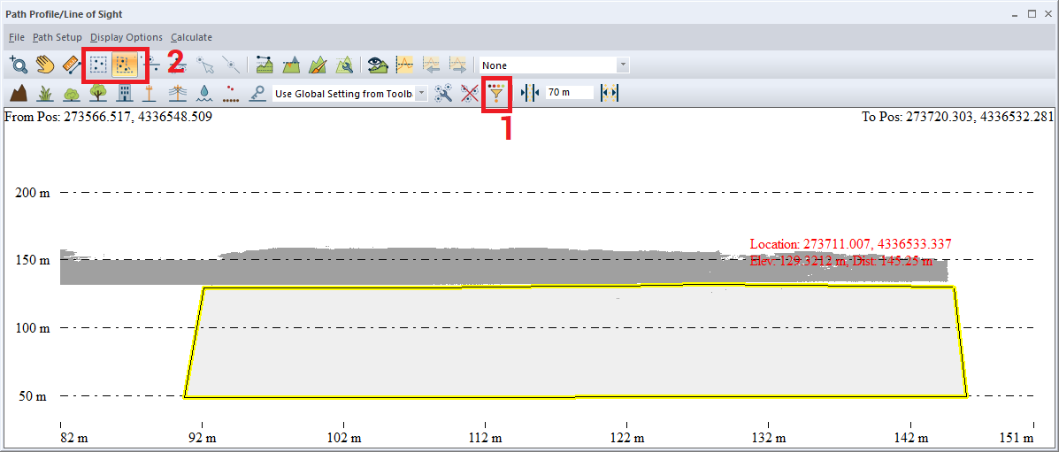
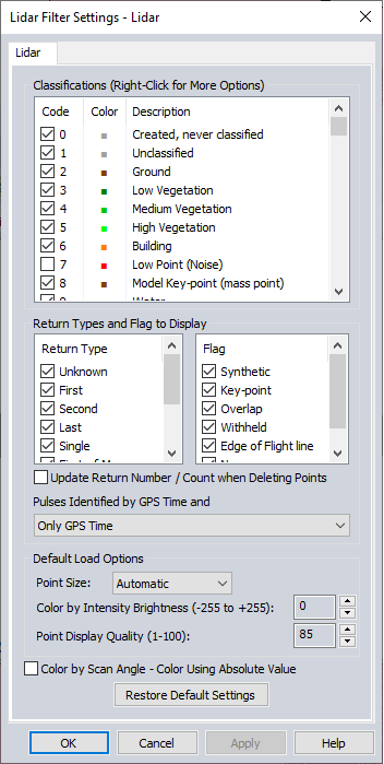
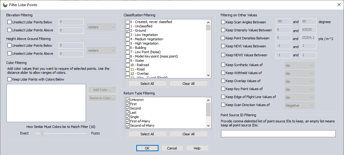
For this click on “Filter Lidar Data” 1 (Figure 15) and in opened window (Figure 16) we remove check marks with “Low Point (Noise)” and “High Point (Noise)”. Click ” Apply ” and then “OK”. This will hide the already filtered noise.
Then click on “Select Lidar by Polygon” and select the areas where noise remains. These points will be marked with red markers.
Figure 15. Selecting an area.
Figure 16. Lidar data display parameters.
Click in the menu “Lidar Analysis” -> “Manual Classification…”. A window with a choice of classes will open (Figure 17). Click on ” High Noise “. As a result, these points will be hidden, because we previously removed the noise classes in the display settings. Repeat the procedure several times to achieve the best result.
Figure 17. Selecting the classification of points as noise that were manually selected.
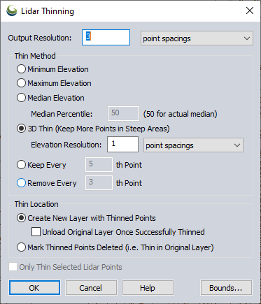
Next, we’ll thin out the cloud a little. For this click on “Lidar Analysis” -> “Spatially Thin Lidar…”. The window that opens will display the layers available for thinning. Make sure that the desired layer is checked and click “OK”.
The window shown in Figure 18 will open. Here you can configure the thinning parameters, which we leave unchanged. Click “OK”. A new thinned layer “area” will be added to the list of layers.
At this stage, it is necessary to separate the ground points from the rest.
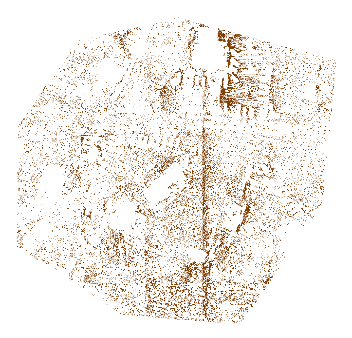
Click on the menu “Lidar Analysis” -> “Automatic Classification” -> “Ground points…”. In the opened panel, set the parameters and click on “Classify Features” (Figure 11). After the classification process is complete, the result can be assessed using 3D viewing by hiding unclassified points in the “Lidar Analysis” -> “Filter Lidar Data…”. In our case, we got the result shown in Figure 19.
Figure 19. Result of classification "Ground Points".
Point Cloud to Digital Elevation Model and Digital Surface Model #
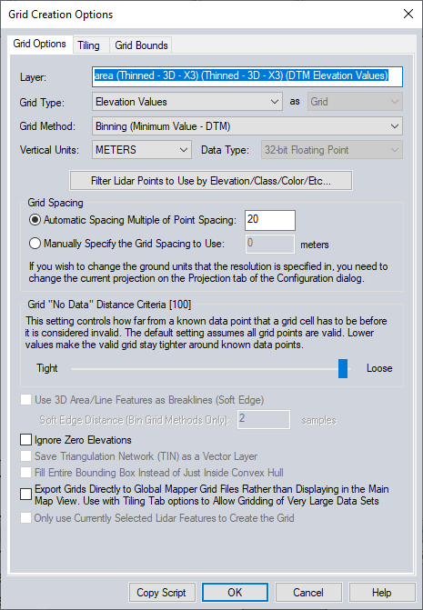
For DEM generation click on “Terrain Analysis” -> “Create Elevation Grid from 3D Vector/Lidar Data…”. In the window that opens, select the layer in which we classified the ground points. Click “OK”. The “Grid Creation Options” window will open, as shown in Figure 20. Here you can configure the DEM generation parameters.
Click on “Filter Lidar Points to Use by Elevation/Class/Color/Etc…”. The window shown in Figure 21 will open. Here we leave the class “Ground” since DEM will be formed from it. Click “OK”.
Figure 20. DEM generation parameters.
Figure 21. Filtering parameters.
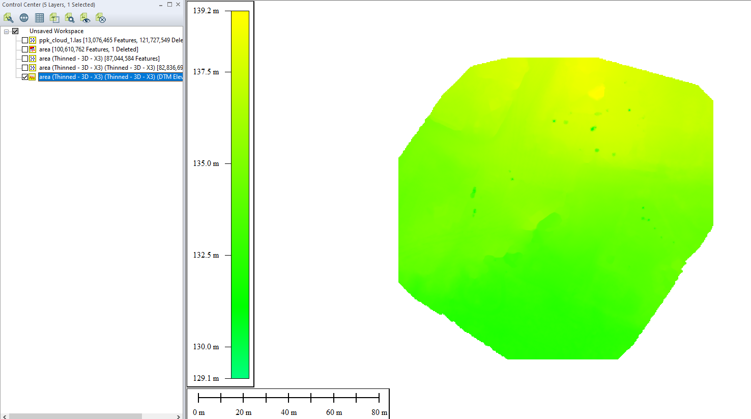
In the “Grid Creation Options” window, click “OK”. You may need to select the “Grid Spacing”, and “Grid ‘No Data’ Distance Criteria” parameters to achieve the best result. The DEM will appear in the viewport and in the layers panel, as shown in Figure 22.
Figure 22. DEM in the viewport.
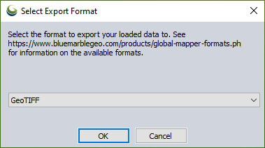
Select DEM in panels layers, and click “File” -> “Export” -> “Raster/Image Format…”. The window shown in Figure 23 will open. Select the format in which you want to save the DEM and click “OK”.
Figure 23. Selecting a file format.
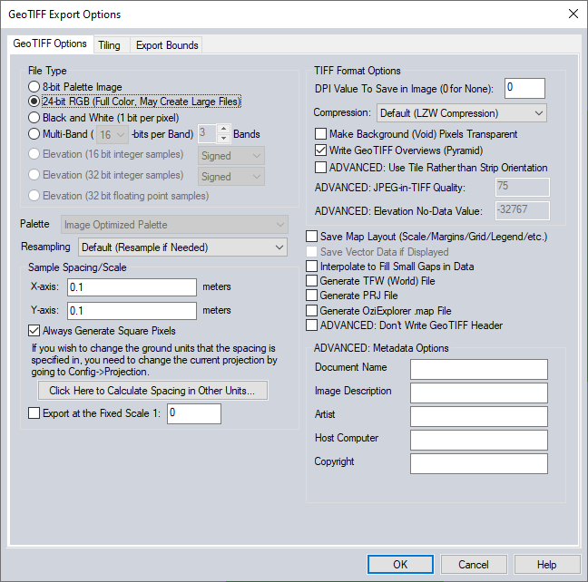
The window shown in Figure 24 will open. Select the desired parameters and click “OK”. A standard save window will open, in which we specify the file name and the path to save the file.
Figure 24. Export parameters.
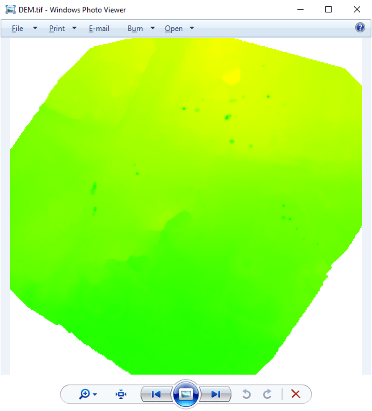
As a result, we obtained the DEM shown in Figure 25.
Figure 25. DEM generation results.
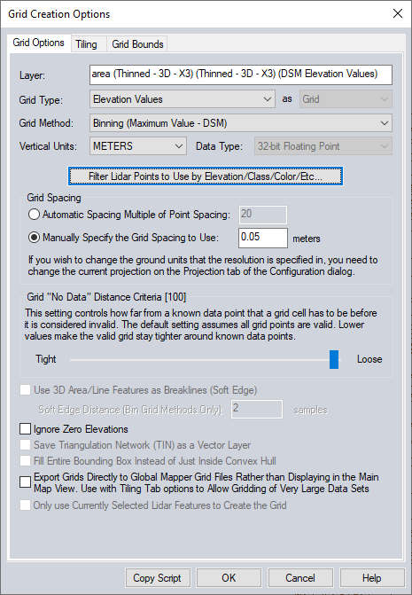
For DSM generation click on “Terrain Analysis” -> “Create Elevation Grid from 3D Vector/Lidar Data…”. In the window that opens, select the layer in which we classified the ground points. Click “OK”. The “Grid Creation Options ” window will open, as shown in Figure 26. Here you can configure the DSM generation parameters.
Click on “Filter Lidar Points to Use by Elevation/Class/Color/Etc…”. A window with filtering parameters will open, as in the case of DEM. Here we leave the class “Ground” and the class “Created, never classified”. Click “OK”.
Figure 26. Parameters for DSM generation.
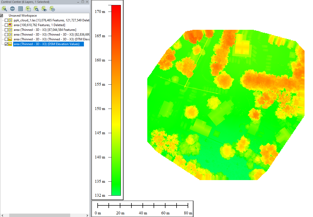
The DSM will appear in the viewport and in the layers panel, as shown in Figure 27.
Figure 27. DSM in the viewing window.
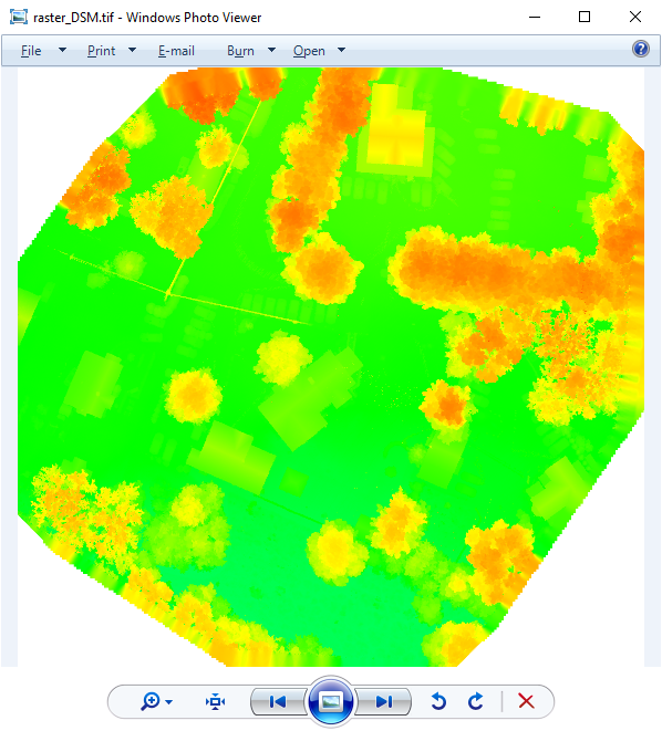
Exporting to a file is done in the same way as with DEM, so we will not describe this procedure again. The result of the DSM generation is shown in Figure 28.
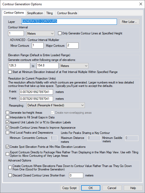
To generate contours, click in the menu “Terrain Analysis” -> “Generate Contours (from Terrain Grid or Lidar)…”. The window shown in Figure 29 will open. Set the parameters for generating contours and click “OK”.
Figure 29. Parameters for generating contours.
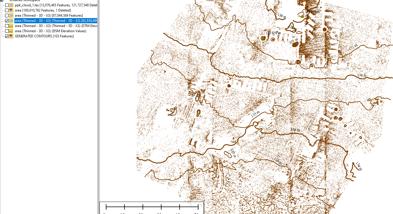
As a result, the contours will be displayed in the layers panel and on the point cloud, as shown in Figure 30. The contours can be saved in a format such as tiff, as well as DSM/DEM.
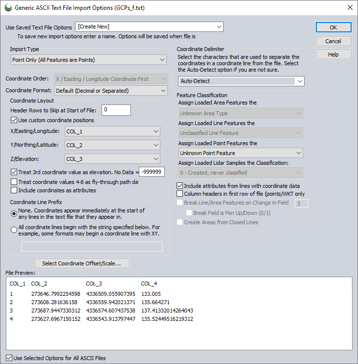
To generate the accuracy report you will need a file with Ground Control Points. Click “File” -> “Open Data File(s)” and select the file with the control points. In our case, it is a regular text file. The window shown in Figure 31 will open. In this window, it is important to correctly configure the column order. Click “OK”.
Figure 31. Control point import parameters.
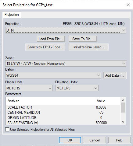
The window shown in Figure 32 will open. Here the projection is configured. In this case, the program automatically determines the correct projection, so we simply click “OK”.
Figure 32. Projection parameters.
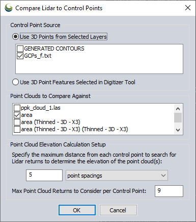
Click on menu “Lidar Analysis” -> “QC Tools” -> “Lidar QC…”. A window will open (Figure 33), where you need to specify the source of control points and the layer that will be compared to assess the accuracy. Click “OK”.
Figure 33. Selecting data for accuracy assessment.
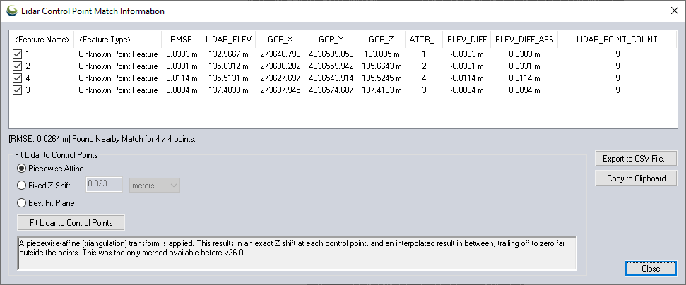
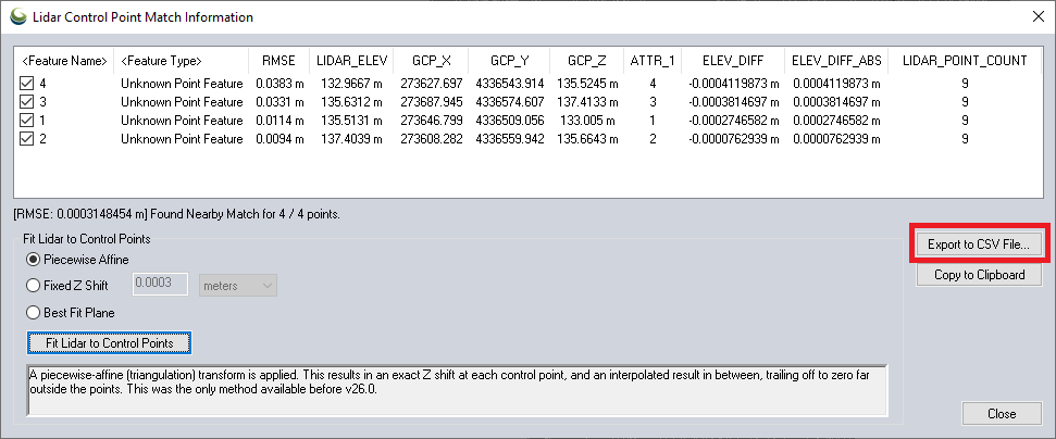
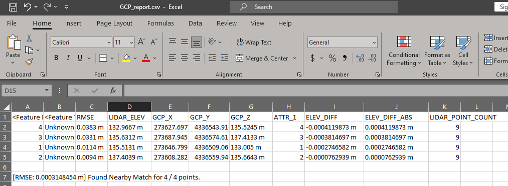
The window shown in Figure 34 will open. As you can see, we have obtained excellent accuracy, since the difference in heights ELEV_DIFF does not exceed 4 cm. You can improve the result by adjusting the error. To do this, click on “Fit Lidar to Control Points”. After correction, the report window will be updated and the generated report can be saved by clicking on “Export to CSV File…” (Figure 35).