Contour lines, the Digital Elevation Model (DEM), and the Digital Surface Model (DSM) are commonly implemented geospatial deliverables created using point clouds. This guide will show how to retrieve these models from a point cloud from RESEPI in Lidar 360 by GreenValley International. We will also look at how to generate reports and show you the key aspects to pay attention to.
Any activity with point clouds begins with the import of data. In LiDAR360, this can be done in several ways:
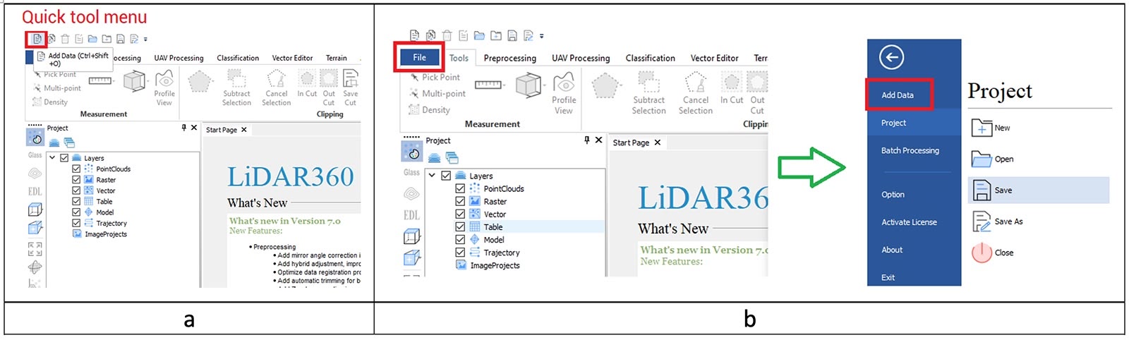
Use the Quick Access menu in the upper-left corner, as shown in Figure 1 a.
As shown in Figure 1 b, click on the “File” button and then click on “Add Data” in the window that opens.
A dialogue box will pop up to specify the path to the .las (.laz) file.
Figure 1. “Add Data” workflow.
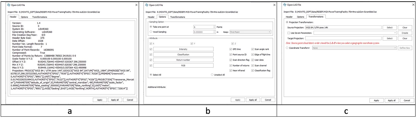
After selecting the file, the program will display header information about the .las (.laz) file in the window shown in Figure 2.
Figure 2. “Open LAS file” window and tabs.
In the additional tabs, you can select the attributes that will be read from the .las (.laz) file, subsample them, or reproject the point cloud to another coordinate system. All attributes are selected by default, there is no subsampling, and the coordinate system is automatically selected according to the point cloud georeferenced.
We’ll leave all these options at their defaults. To load the point cloud, click on “Apply”.
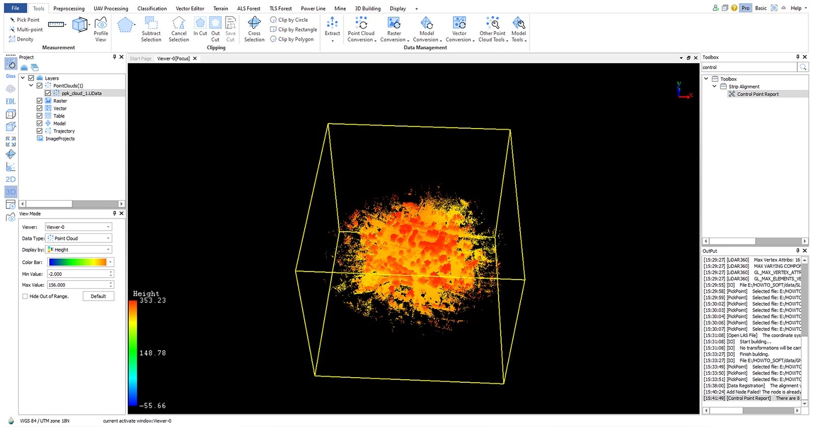
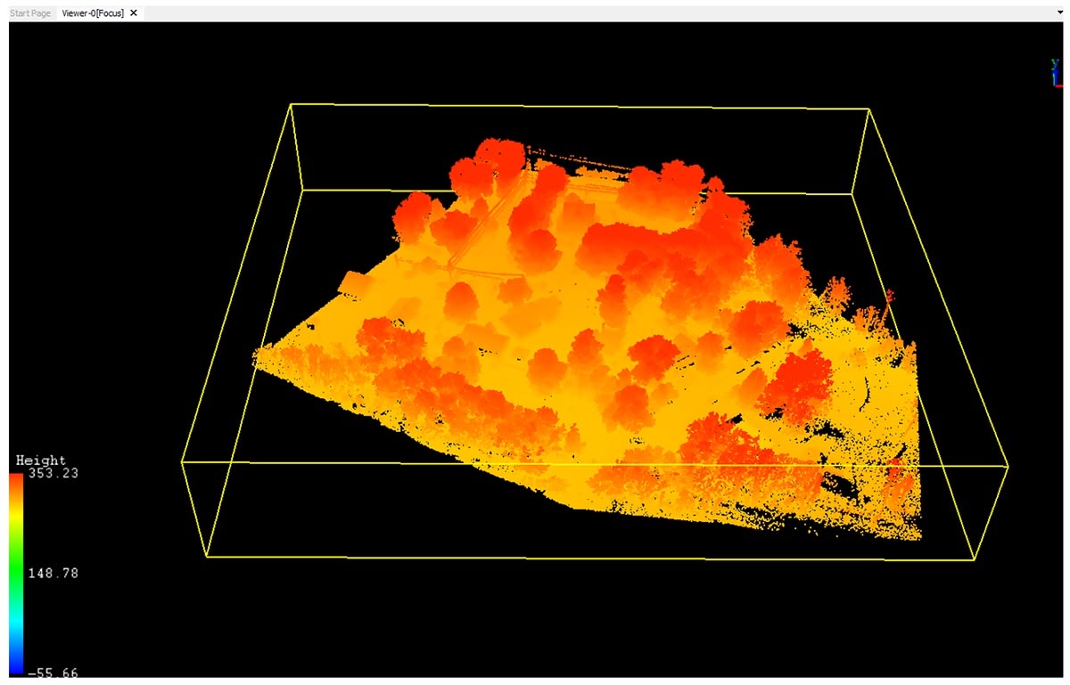
As a result, our point cloud will be displayed in the main window, as shown in Figure 3.
The next step is to prepare the point cloud for DSM, DEM, and Contours. To do this, we’ll use the crop tool to remove unrequired points and thin out the clouds. This step will also speed up data processing.
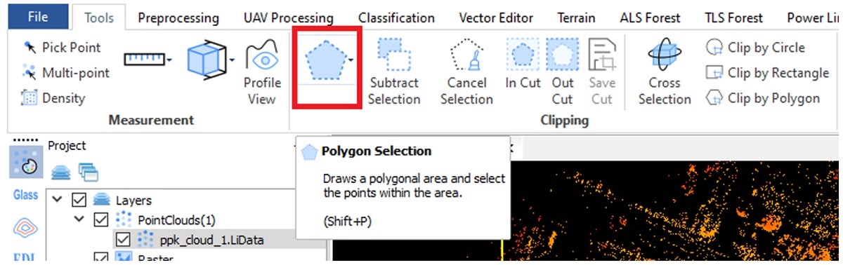
To remove the extra points, click on the “Selection” tool in the “Clipping” panel (Figure 4).
Figure 4. “Polygon Selection” tool in the “Clipping” panel.
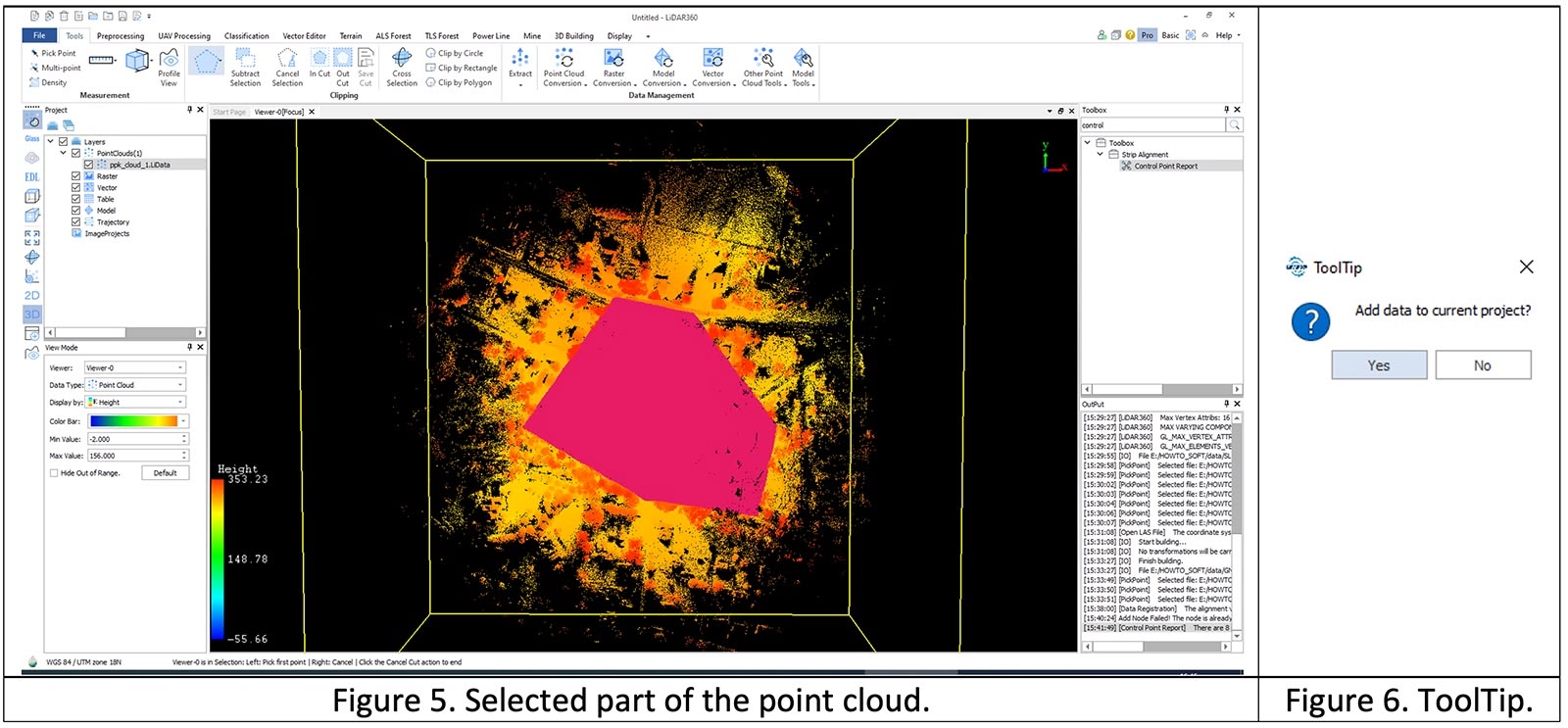
After selecting the desired area, it will be highlighted in pink, as shown in Figure 5.
To delete the selected fragment, click “In Cut”. This step will remove any UNSELECTED points.
To delete the selected fragment, click “Out Cut”.
We are interested in the selected fragment in this case, so we click “In Cut”.
After cutting off the excess, click “Save Cut to save the fragment.
The program will save the fragment and prompt to add it to the current project, as shown in Figure 6. Click “Yes”.
The next step is to subsample and remove the noise/outliers, Figure 6.
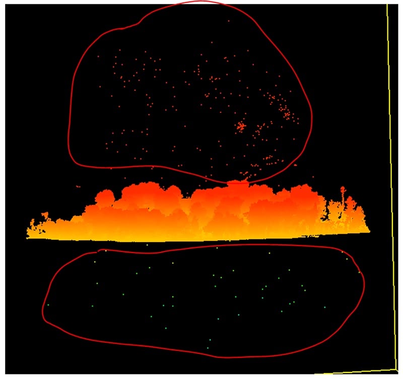
Figure 7. Outliers.
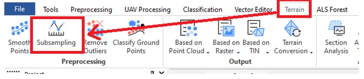
To subsample the point cloud, go to the “Terrain” tab and click “Subsampling” as shown in Figure 8.
Figure 8. Subsampling tool.
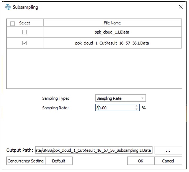
The Subsampling Options window opens as shown in Figure 9.
Figure 9. “Subsampling” parameters.
Ensure that the desired point cloud is selected, select the desired sampling type and rate, and click “OK”.
After subsampling, remaining outliers can be removed using the “Selection” tool.
After we removed the outliers and thinned out the data a bit, we had a ready-made cloud for classification, Figure 10.
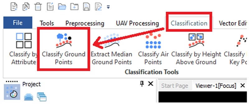
To classify points, go to the “Classification” tab and click “Classify Ground Points”, Figure 11.
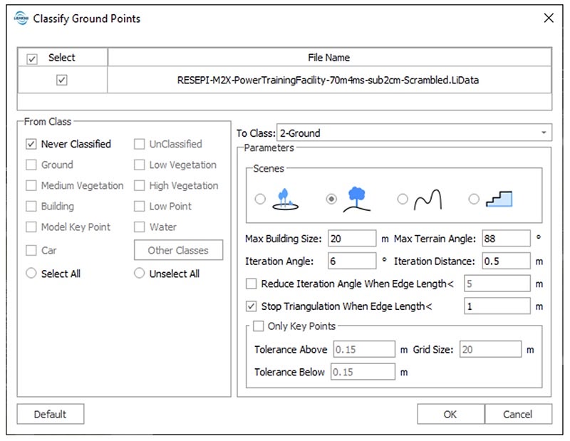
In the “Classify Ground Points” parameters window that opens, we need to select the ‘From Class” option and select the ‘Select All’ option to ensure that all the data points are chosen to be classified as ground.
Select the surface type and adjust the necessary parameters as shown in Figure 12. In our case, the area has small hills, so we chose “Gentle Terrain”. The rest of the parameters are left as they are.
Figure 11. “Classify Ground Points” workflow.
Figure 12. “Classify Ground Points” parameters.
Click “OK” to start the classification of land-based points.
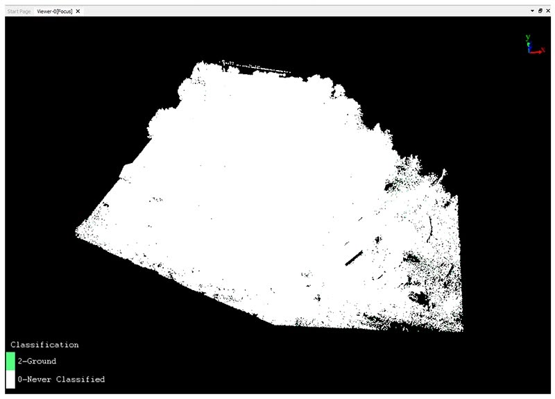
Once the classification process is complete, the point cloud will look like Figure 13.
Figure 13. Classified point cloud.
To see the result, you need to do the following:
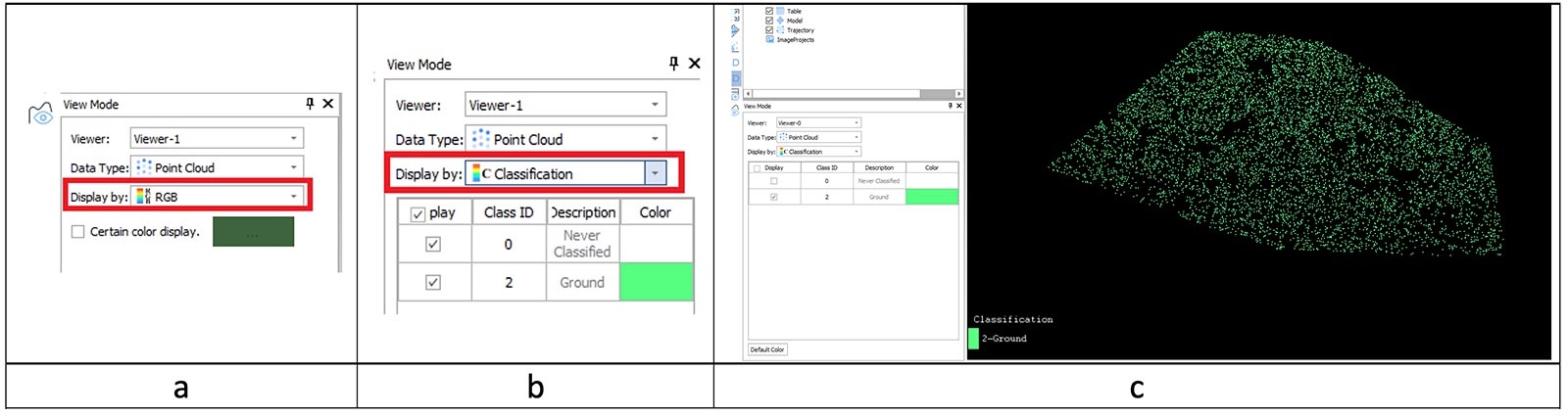
In the “View Mode” window, select “Displayed by Classification” as shown in Figure 14 a, b.
Hide unclassified points by unchecking the display options for “Never Classified” points, Figure 14 c.
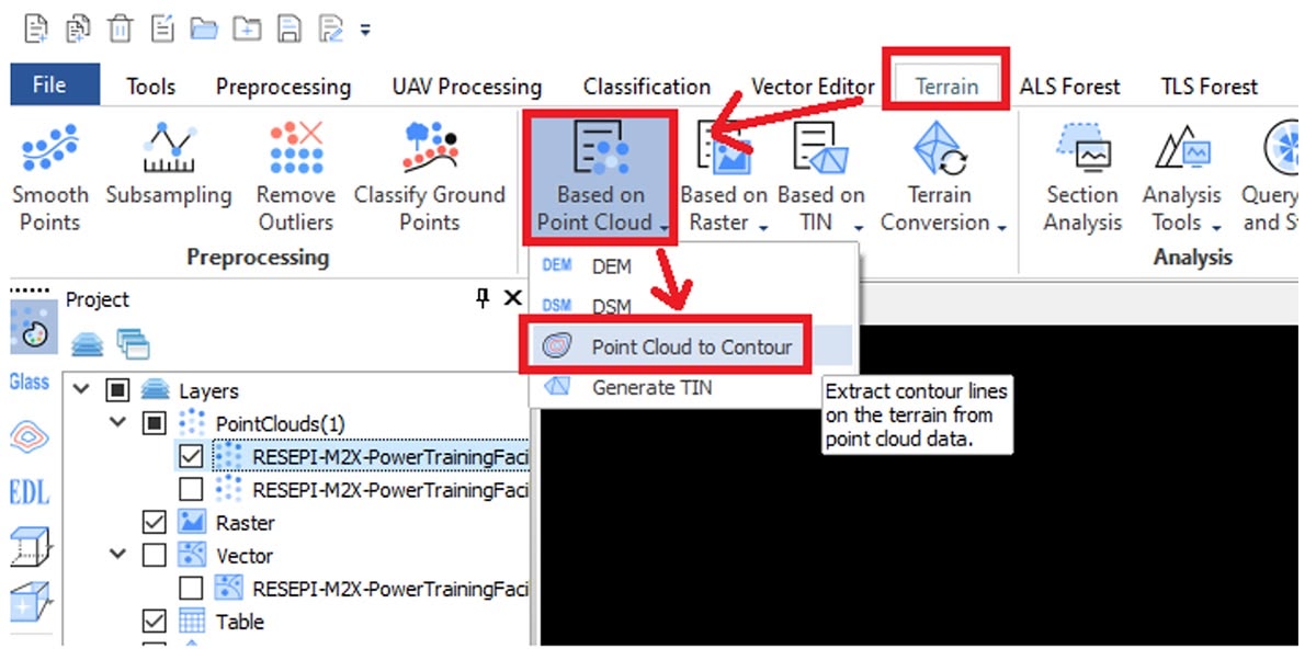
Go to the “Terrain” tab and click “Based on Point Cloud”, ass shown in Figure 15.
Select the “Point Cloud to Contour” option.
Figure 15. “Point Cloud to Contour” workflow.
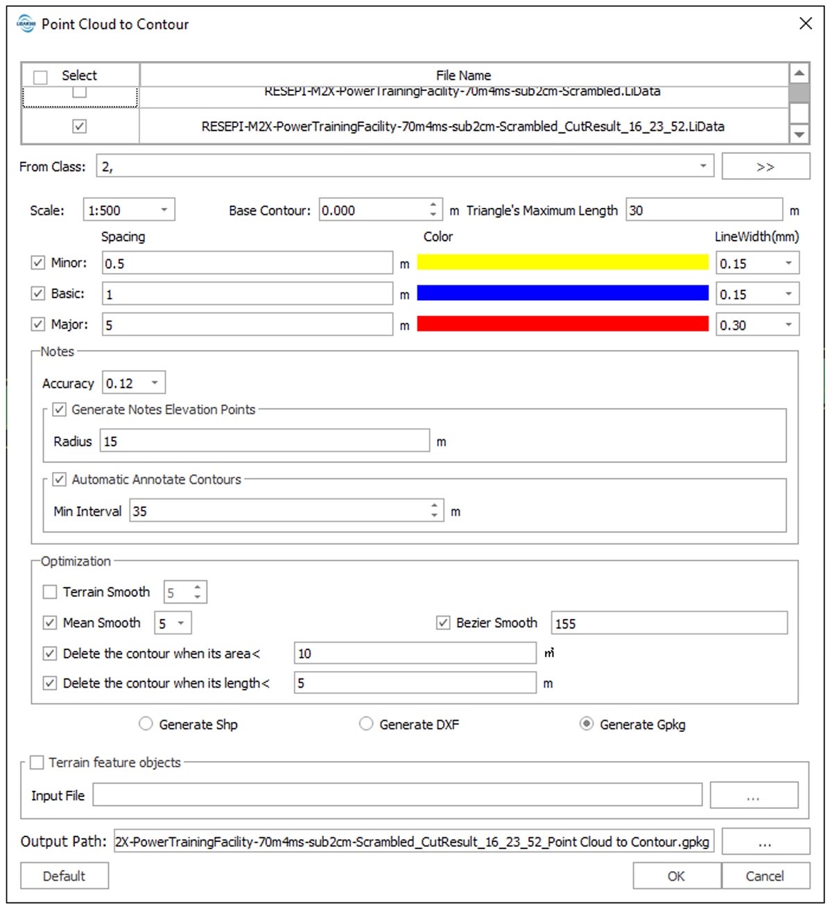
The Point Cloud to Contour parameters window opens, as shown in Figure 16. Leave the default settings and click “OK.”
Figure 16. “Point Cloud to Contour” parameters window.
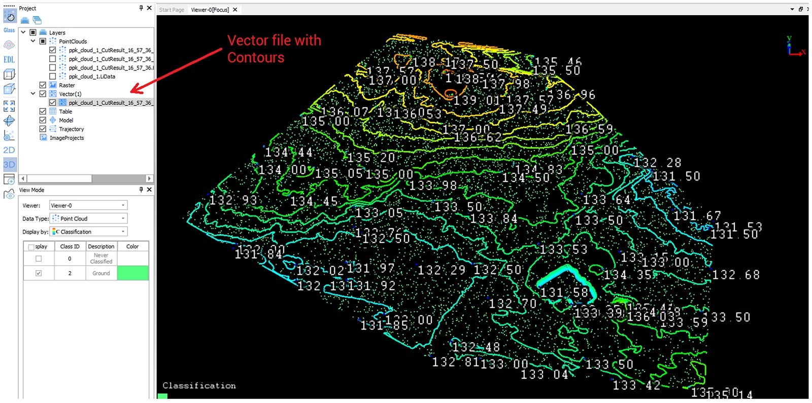
As a result, a file will appear in the “Vector” section that stores information about the paths. The contours drawn on the point cloud will then be visible on the point cloud, as shown in Figure 17.
Figure 17. Contours on a point cloud.
Point Cloud to Digital Elevation Model and Digital Surface Model #
Digital map generation is the same as in the case of contour generation, Figure 15:
To get a DEM, go to the “Terrain” tab and click “Based on Point Cloud”.
Select the ‘DEM’ option.
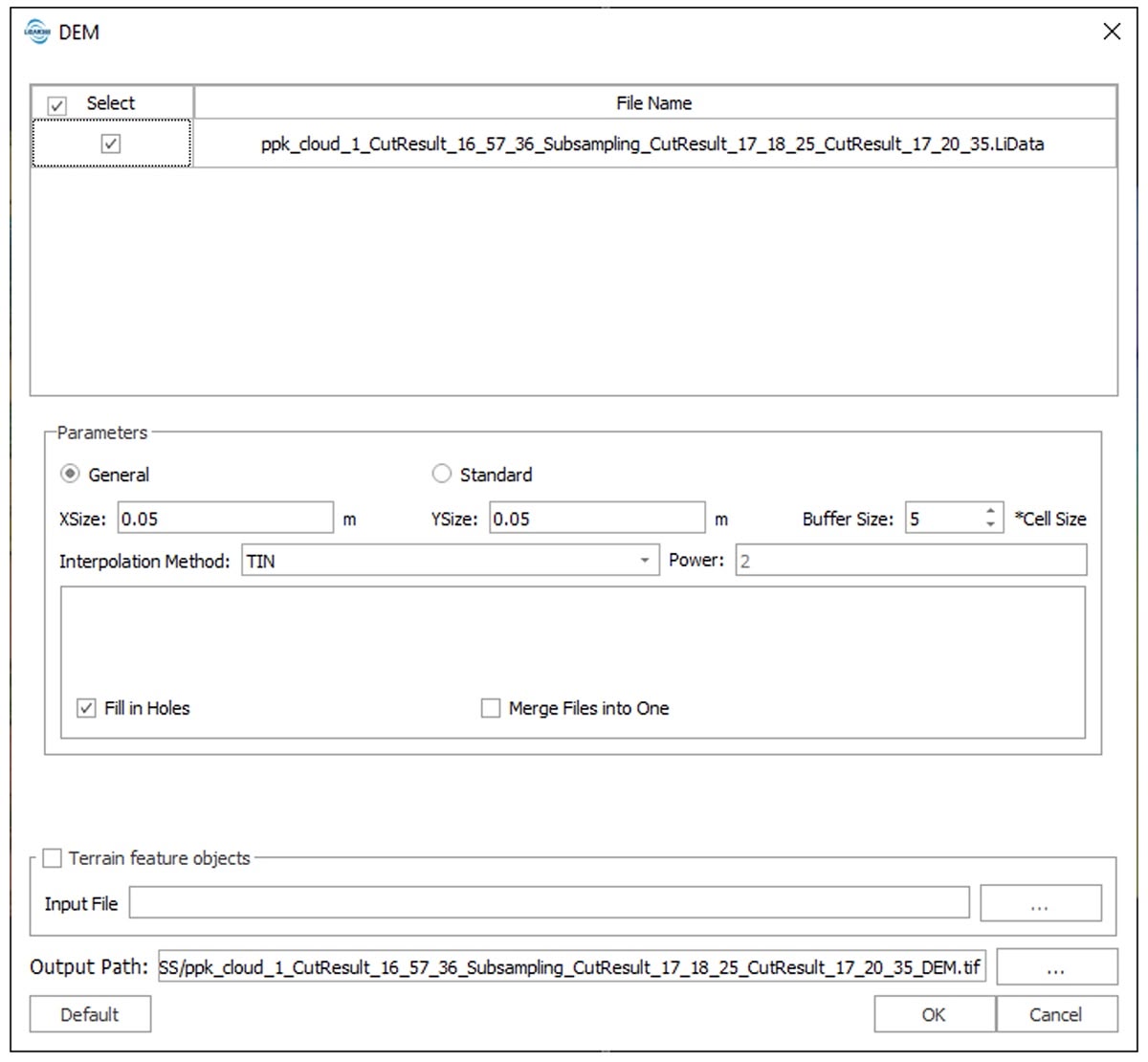
A window opens with the DEM generation parameters, as shown in Figure 18.
Figure 18. “DEM” parameters.
Required mesh resolution and the interpolation method can be configured here.
For the detailed map, let’s choose the grid size “XSize” and “YSize” equal to 0.05 m.
To fill the gaps, select the “TIN” method and check the “Fill in Holes” box, then click “OK”.
The result is a DEM as shown in Figure 19.
DSM generation occurs similarly:
To get DSM, go to the “Terrain” tab and click on “Based on Point Cloud”.
In this case, we will need the “DSM” tool.
A window opens with the DSM generation parameters, as shown in Figure 19.
For the detailed map, we will choose the grid size “XSize” and “YSize” equal to 0.1 m.
To fill the voids, select the “Delaunay” method and check the “Fill in Holes” box, then click “OK”.
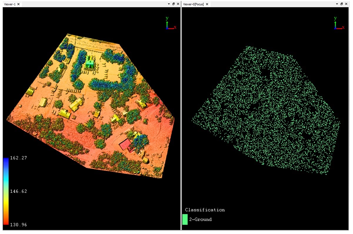
The result is a DSM, as shown in Figure 20.
Figure 20. Point cloud (right) and DSM (left).
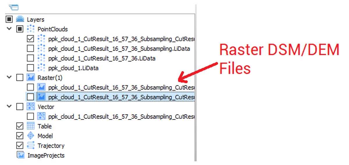
Once the DSM and DEM are generated, they will be displayed in the “Raster” tab, Figure 21.
Figure 21. DSM and DEM Raster files.
Now let’s move on to a very important section: Reports. After processing the data and receiving the maps, you need to make sure that they are suitable for use. For this, LiDAR360 has convenient reporting tools.
The Control point report tool outputs an accuracy report between the point cloud and the independently surveyed control points and checkpoints. These values can then also be used to manually register the point cloud to the desired altitude values.
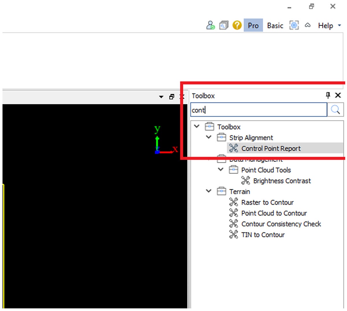
The first report we’ll look at is the “Control Point Report”, which can be found in the “Toolbox” tab.
For a quick search, you can use the search bar by typing the name of the toolbox, Figure 22.
Figure 22. “Control Point Report” in the “Toolbox” tab.
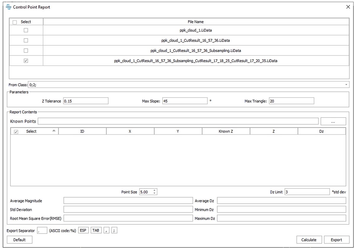
The toolbox is launched by double-clicking on it, after which you will see the window shown in Figure 23.
Figure 23. “Control Point Report” toolbox.
Here it is important to pay attention to the “Report Contents” and the “Average magnitude”, “Std Deviation”, and “Root Mean Square Error (RMSE)” display fields. They will display information about the accuracy of the point cloud.
From the “From Class” field, select only the ‘02’ option as it chooses the ground classified points only and not all the points which would include points not on the ground as well.
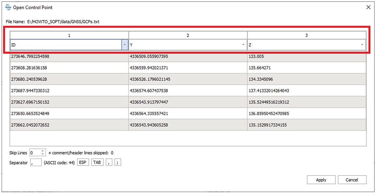
To load checkpoints, click on the button with three dots next to the “Known Points” field. A window, shown in Figure 24, opens.
If necessary, you can change the type of column according to the data. By default, the first column is assigned as the point number. In our case, it is not in the text file, so we replace the first column in the drop-down list with “X”, the second and third will be the coordinates “Y” and “Z”, respectively, Figure 25.
Figure 24. “Open Control Point” window.
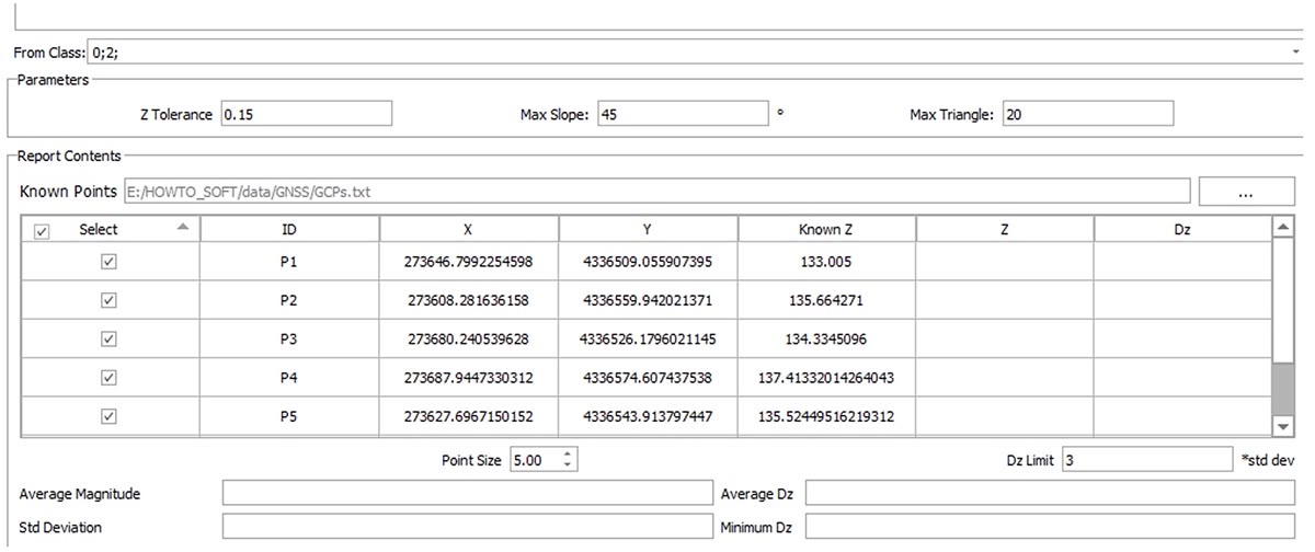
After the setup, click on “Apply”. The Open Control Point window closes, and we see a list of control points in the Control Point Report window, Figure 26.
Figure 25. Correct loading of checkpoints.
Figure 26. A list of checkpoints.
In this case, we will leave the parameters by default. We will only note that:
Z tolerance (default value is “0.15”): The accuracy of the point cloud in the Z-axis direction. To avoid the distance between the points being too small leading to an excessive slope.
Dz limit (default value is “3”): Set the tolerance of Dz. If Dz is not within the tolerance, show red to inspect the elevation difference with a large error between the point cloud and control points. Maximum tolerance = Average Dz + Dz * Std Deviation. Minimum tolerance = Average Dz – Dz * Std Deviation
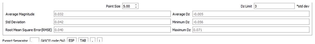
To start the calculation, click on the “Calculate” button in the lower right corner of the window.
The result is a report on the accuracy of our scan, Figure 27.
Figure 27. Point cloud Z-accuracy report.
To export the report to a file, click on “Export”. A save window will open, where you specify the path where you want to save the report.
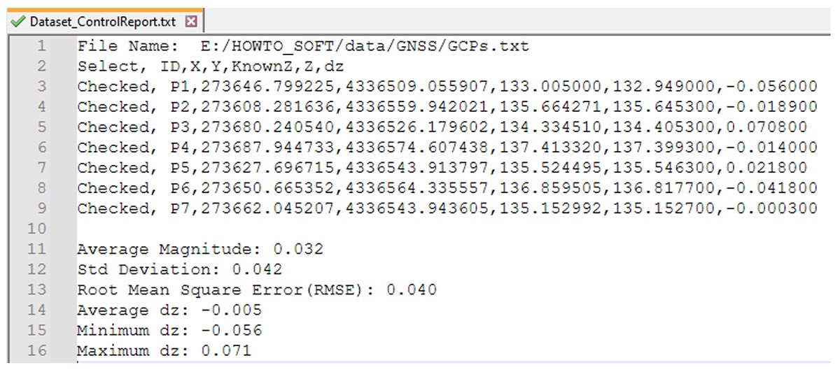
The report will contain information about the control points and the results of the calculated accuracy, as shown in Figure 28.
Figure 28. Z-Accuracy report.
Now let’s look at the DSM/DEM report generation that we generated earlier.
To create a report, use the “Toolbox” menu and its search bar. The toolbox we need is called “DEM Accuracy Assessment”, as shown in Figure 29.
Figure 29. “DEM Accuracy Assessment” toolbox.
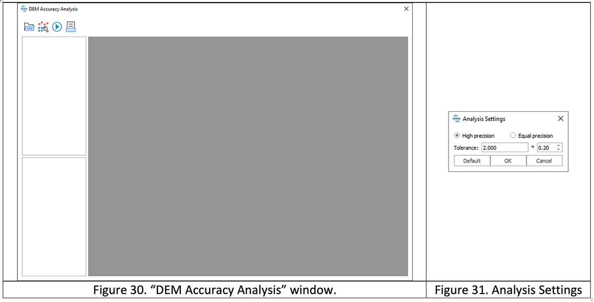
After opening the toolbox, the DEM Accuracy Analysis window, Figure 30 opens. At the top left, there are buttons for loading data and running calculations:
button opens the .tiff file selection window.
button opens the checkpoint loading window.
button starts the process of calculating accuracy.
button opens the window for saving the report.
To create a report, you need to open a .tiff file, load checkpoints, run the report, and then export it.
After starting the calculation process, a window will open that will prompt you to select the precision, Figure 31.
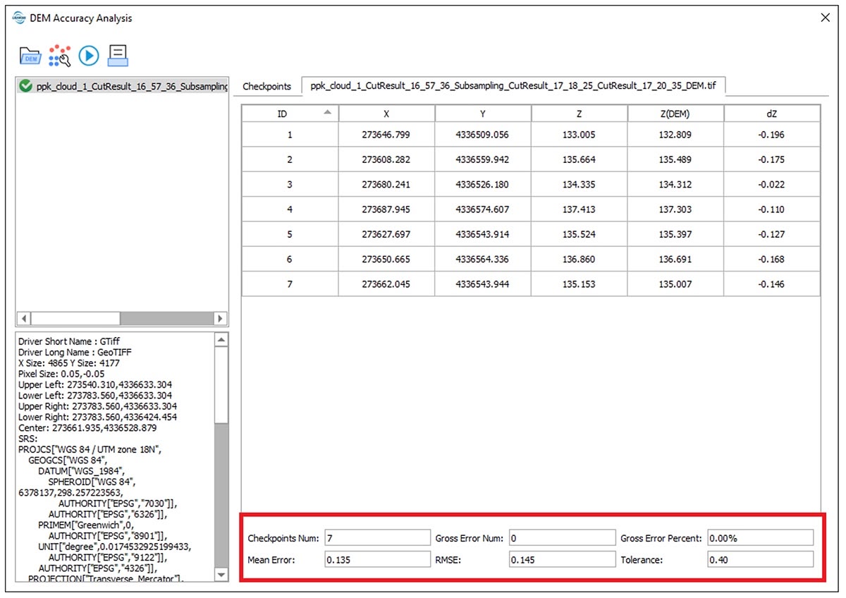
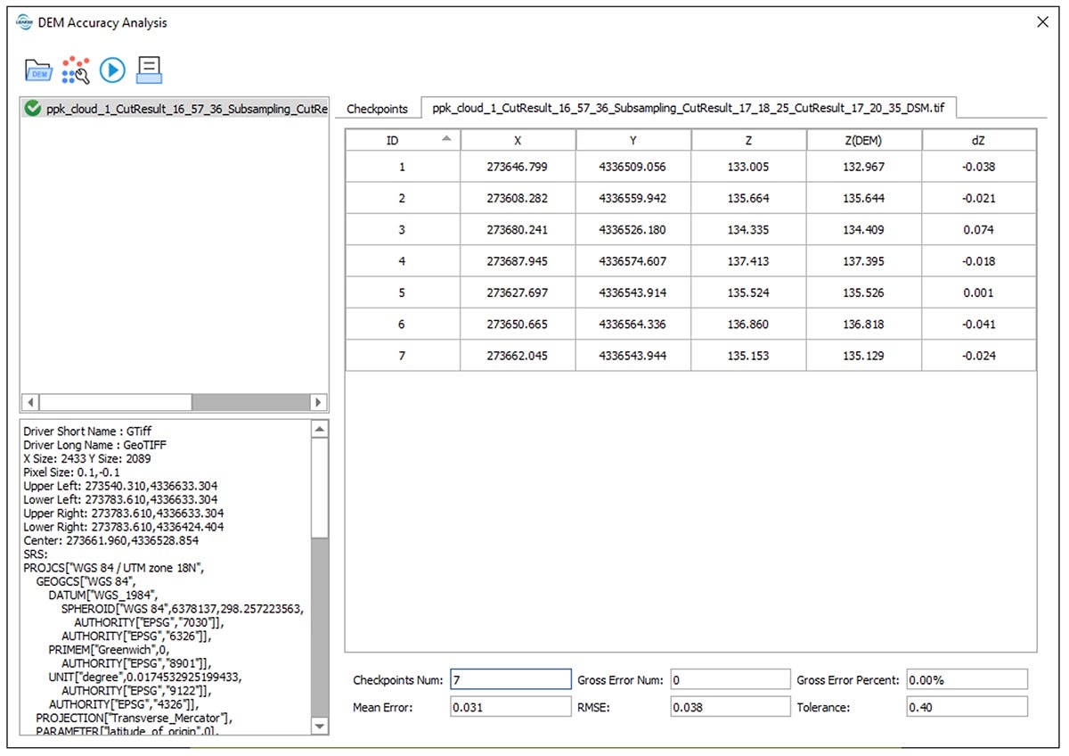
As a result, we will get the accuracy data of our DEM, Figure 32.
Figure 32. Result. ( indicates the digital elevation model error The gross error rate is less than 5%).
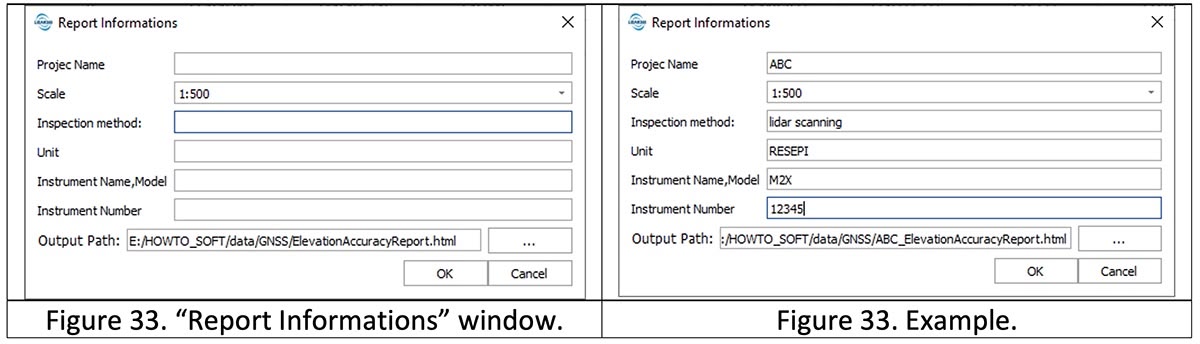
To export, click on and enter the data in the “Report Informations” window, Figure 33.
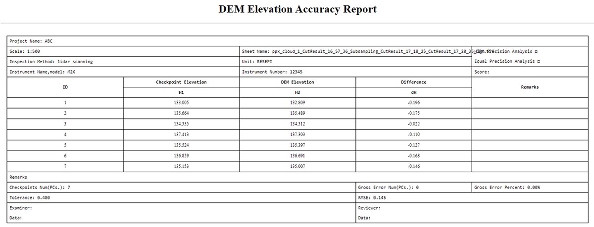
Click “OK” and open the report. In this case, it is a .html file that can be opened in any web browser, Figure 34.
Figure 34. DEM Accuracy report.
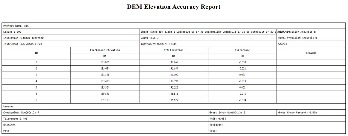
Similarly, you can generate a report for a DSM file, Figure 35, 36.