An aerial and ground survey can obtain a full terrain scan. Most often, aerial surveys are carried out using GNSS, which results in georeferenced data after the flight. The ground part is often scanned in SLAM mode. Thus, the ground scan data has local coordinates. To combine both datasets, georeferencing of SLAM data is necessary. And this can be a big problem, especially for beginners of LiDAR payloads. But in fact, it is very simple. This guide will show how to georeference SLAM point cloud data from RESEPI in LiDAR360 by GreenValley International. We will also look at how to generate reports and show you the key aspects to pay attention to.
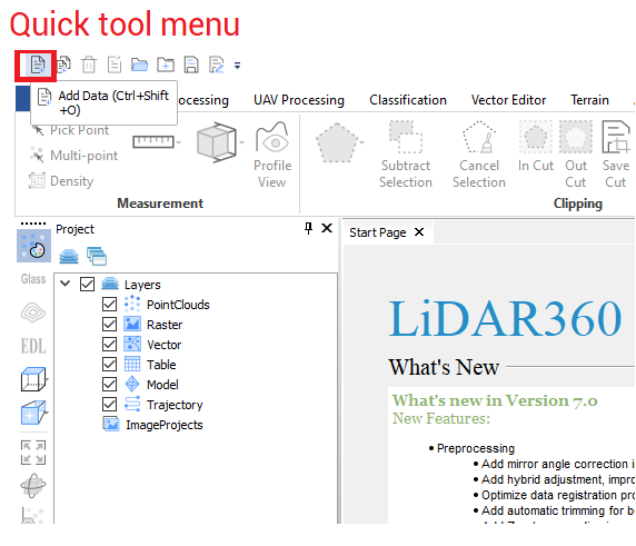
Any activity with point clouds begins with the import of data. In LiDAR360, this can be done in several ways:
Use the Quick Access menu in the upper-left corner, as shown in Figure 1 a.
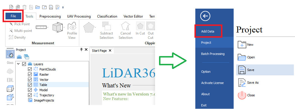
Click on the “File” button, and then click on “Add Data” in the window that opens, as shown in Figure 1 b.
This will open a window where you need to specify the path to the .las (.laz) file.
Figure 1a. “Add Data” workflow.
Figure 1b. “Add Data” workflow.
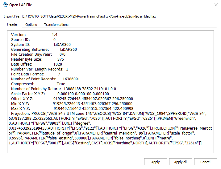
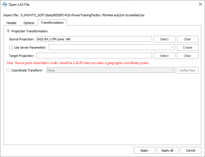
After selecting the file, the program will display information about the .las (.laz) file in the window shown in Figure 2 a,b,c.
Figure 2a. “Open LAS file” window and tabs.
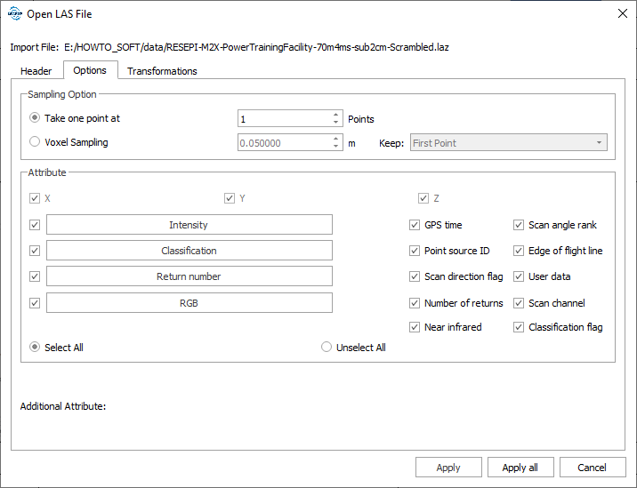
Figure 2b. “Open LAS file” window and tabs.
Figure 2c. “Open LAS file” window and tabs.
In the additional tabs, you can select the attributes that will be read from the .las (.laz) file, thin, or reproject the point cloud to another coordinate system. By default, all attributes are selected, there is no thinning, and the coordinate system is automatically selected according to the point cloud georeferenced.
We’ll leave all of these options at their defaults. To load the point cloud, click on “Apply”.
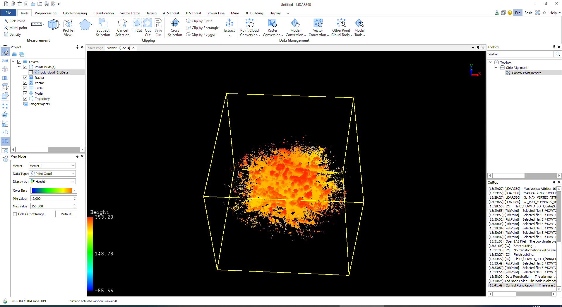
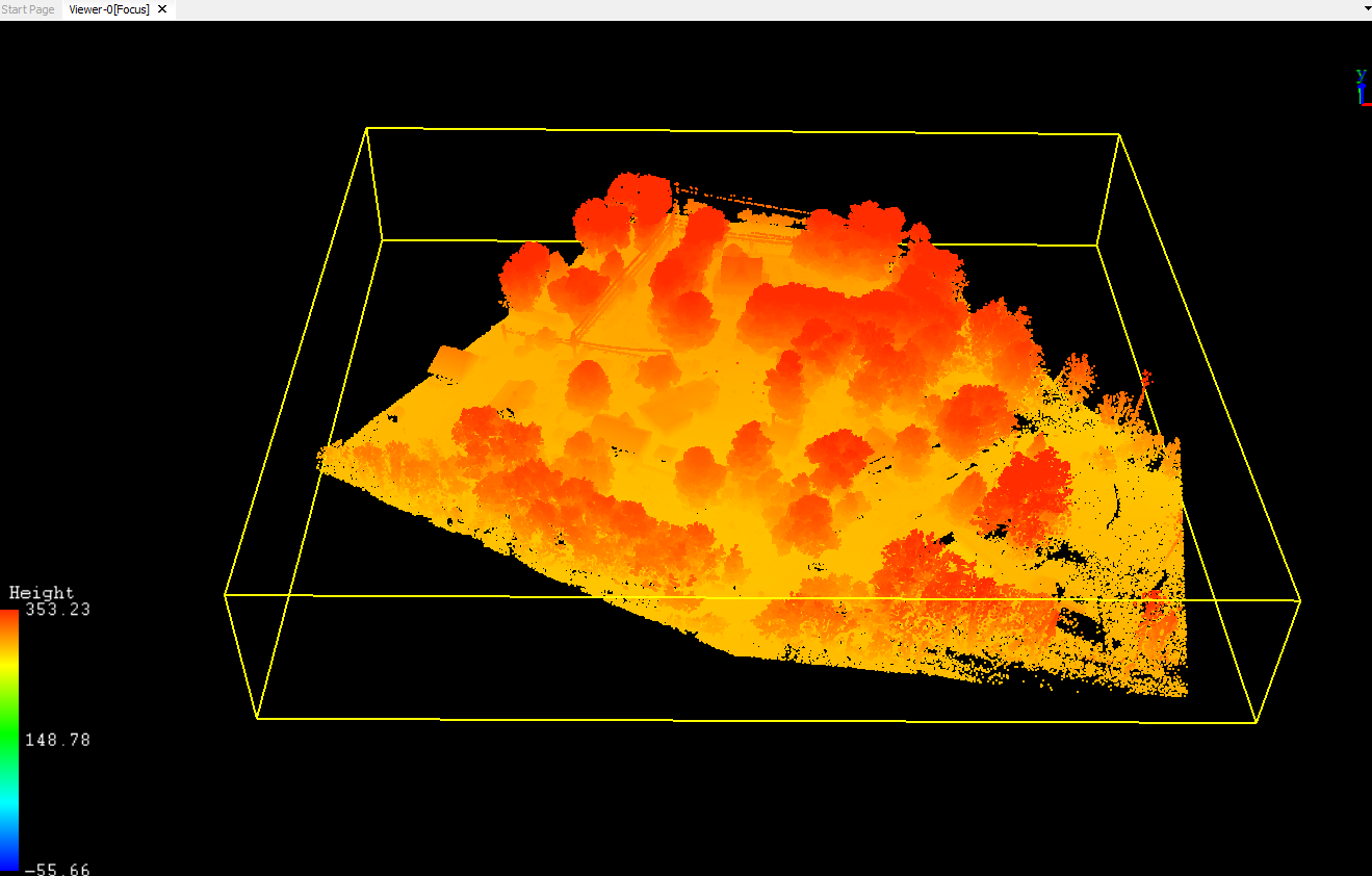
As a result, our point cloud will be displayed in the main window, as you can see in Figure 3.
Figure 3. A loaded point cloud.
Preprocessing point cloud The next step is to prepare the point cloud for georeferencing. To do this, we will use the crop tool to remove unnecessary points and also thin out the cloud. This will also speed up data processing.
In addition, it will speed up data processing.
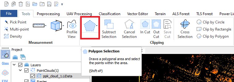
To remove unnecessary points, click on the ‘Selection’ tool in the “Clipping” panel, as shown in Figure 4.
Figure 4. “Polygon Selection” tool in the “Clipping” panel
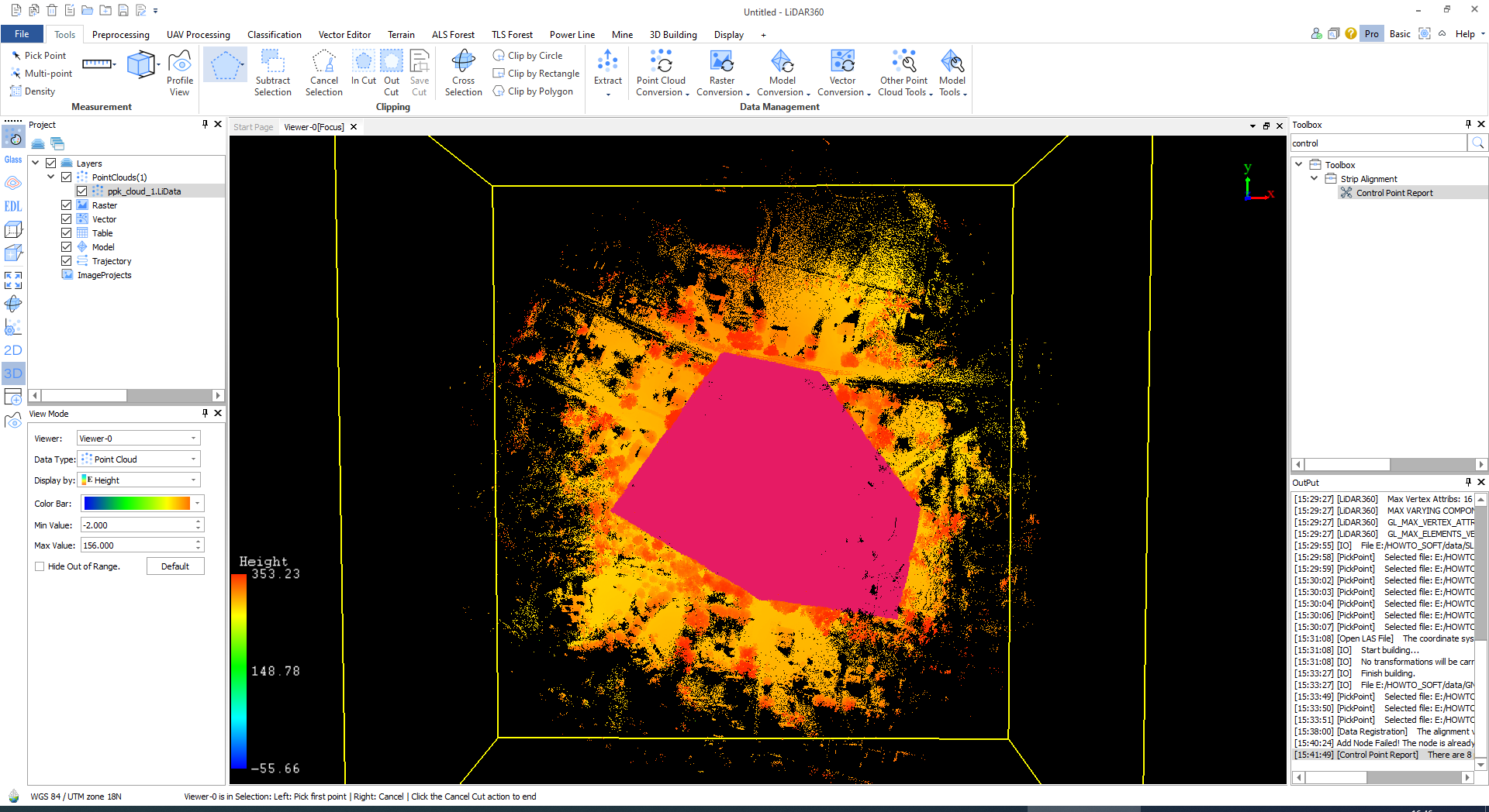
After selecting the desired area, it will be highlighted in purples shown in Figure 5.
If we want to keep only the selected fragment, we need to click “In Cut”. This will remove any UNSELECTED points.
If we want to delete the selected fragment, then we need to click on “Out Cut”.
Since we need only the selected fragment, we click “In Cut”.
After cutting off the excess, you need to save the fragment. To do this, just click on “Save Cut”
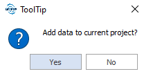
The program will save the fragment and prompt you to add it to the current project, Figure 6. Click on “Yes”.
Figure 5. Selected part of the point cloud.
Figure 6. ToolTip.
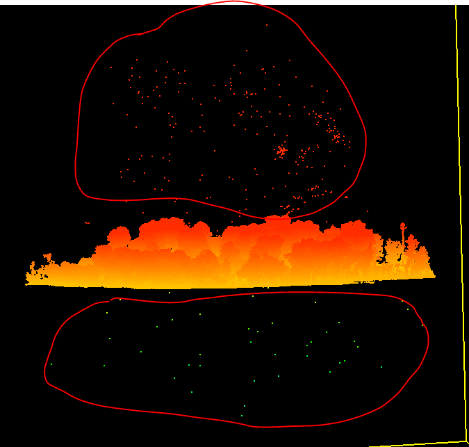
The next step is to thin out and remove the outliers, Figure 7.
Figure 7. Outliers.
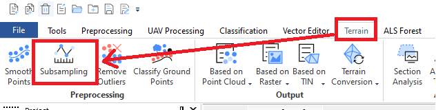
To thin out, go to the “Terrain” tab and click on “Subsampling”, Figure 8.
Figure 8. Subsampling tool.
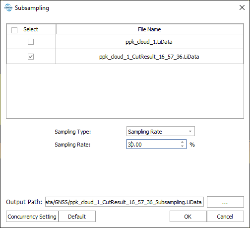
The Subsampling Options window opens, in Figure 9.
Figure 9. “Subsampling” parameters.
Make sure that the correct point cloud is selected, then choose the appropriate thinning type and subsampling value from the drop-down list.
After subsampling, some of the outliers will remain, they can be easily removed with the “Selection” tool
After we removed the outliers and thinned out the data a bit, we had a ready-made cloud for georeferencing, Figure 10.
Figure 10. Prepared point cloud.
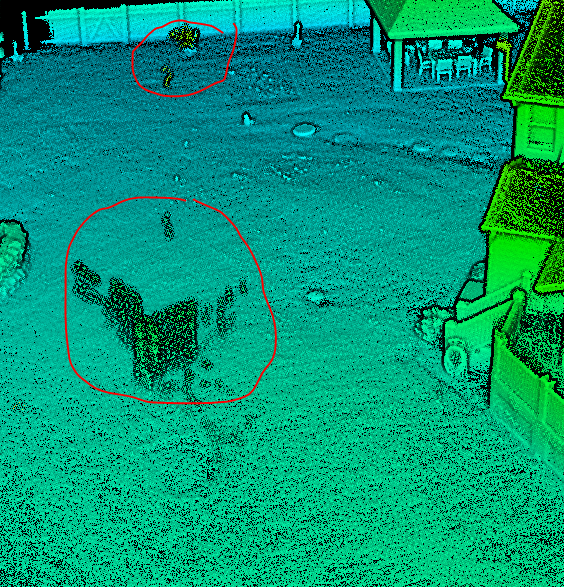
The SLAM point cloud is processed similarly, but due to the nature of SLAM algorithms, additional filtering may be required. Moving objects can leave trails in the point cloud. This can be the flight of birds, the movement of people, etc., as shown in Figure 11.
Figure 11. Trails on SLAM point cloud.
We will consider additional tools that will help to get rid of trails and outliers. To do this, you need to do the following:
In the same way as for the GNSS cloud, we load the SLAM cloud and cut off the excess, and thin out the data (if necessary).
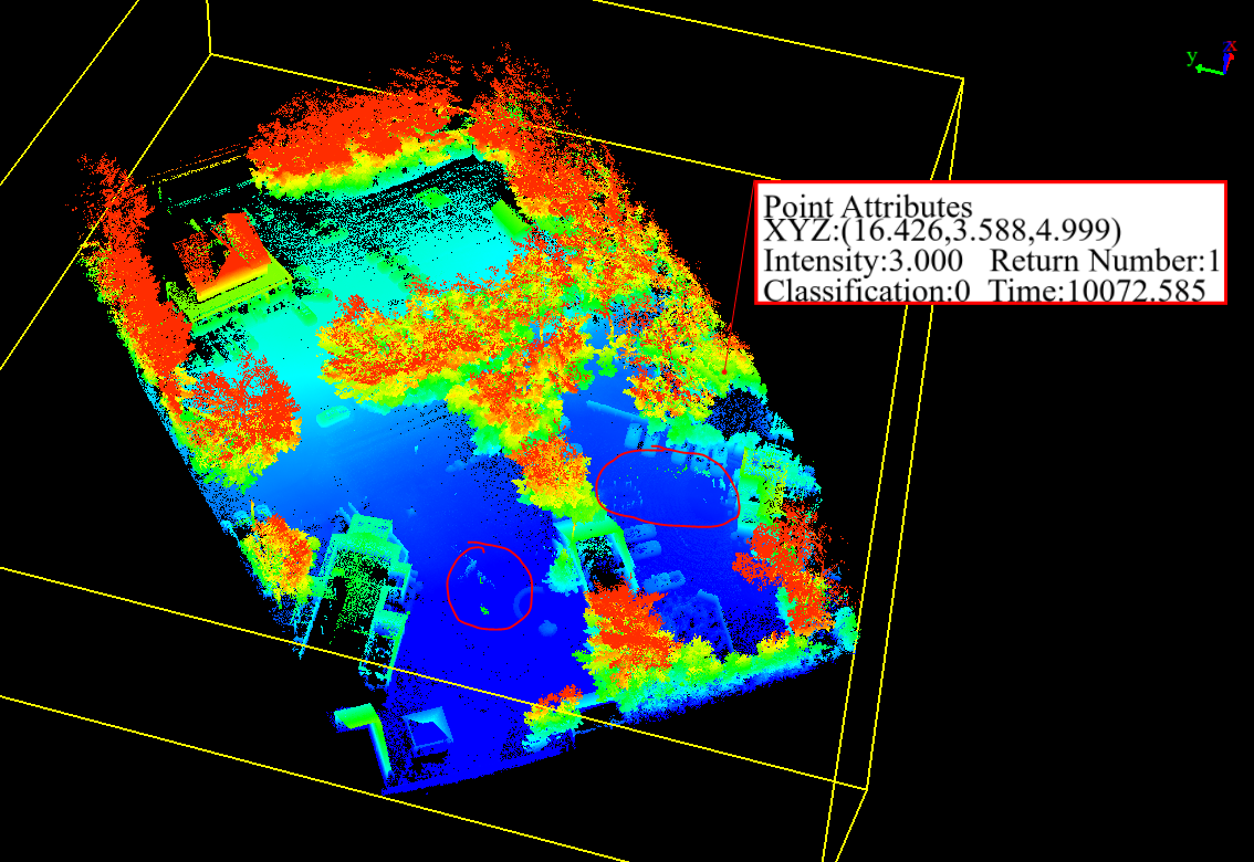
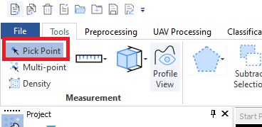
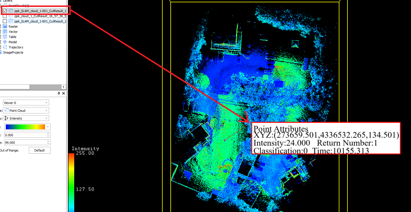
For example, we will show the SLAM cloud in Figure 12. As you can see, we used the “Pick Point” tool, which is available in the top toolbar, Figure 13. Just click on this tool and then at any point in the cloud to find out its coordinates and additional information, which is not worth paying attention to now.
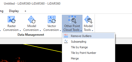
As you can see, there are small trails in the cloud. To get rid of them, we will use the “Remove Outliers” tool, Figure 14.
Figure 12. SLAM cloud with small trails.
Figure 13. «Pick Point» tool.
Figure 14. “Remove Outliers” tool.
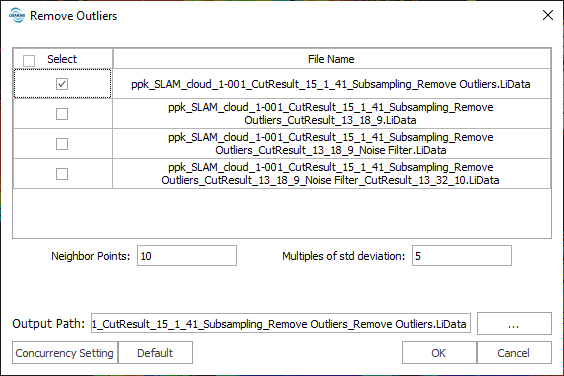
Click on “Remove Outliers”, and a window will open with parameters for removing Outliers, as shown in Figure 15. In this case, we will use the default parameters.
Figure 15. “Remove Outliers” parameters.
Make sure that the desired point cloud is selected and click “OK”. After processing, you will be asked to add data to the project, agree, and evaluate the result, Figure 16.
Figure 16. Result of removing outliers.
As you can see, the trails have been removed and we can proceed to georeferencing.
For convenience, we will leave only processed GNSS and SLAM point clouds in the layers panel, as shown in Figure 17.
Figure 17. We leave only prepared point clouds for the convenience of further work.
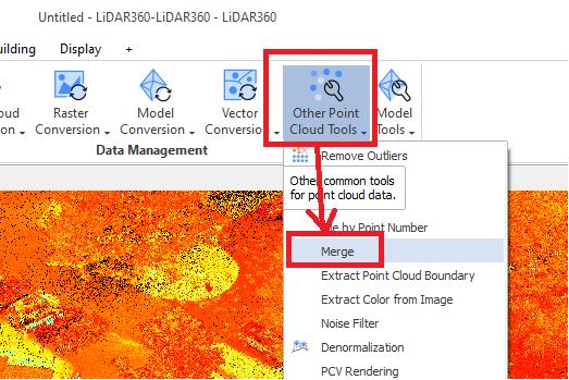
To make georeferencing, we will use the “Data Registration” tool in the “Preprocessing” tab, Figure 18.
Figure 18. “Data Registration” tool.
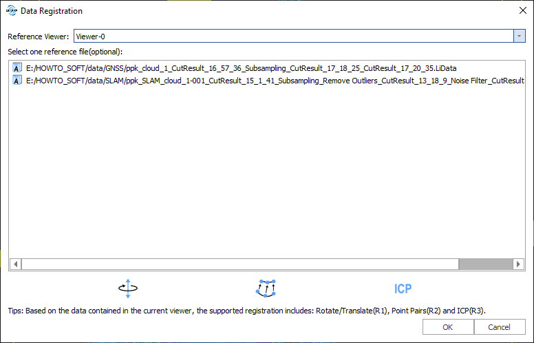
Click on “Data Registration” in the “Preprocessing” tab, and a window will appear, which is shown in Figure 19.
Figure 19. “Data Registration” window.
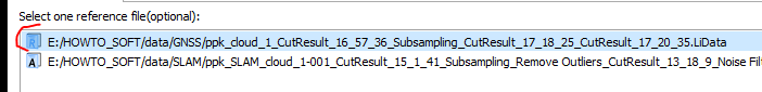
The window offers to select a reference cloud TO WHICH we want to link another cloud. Click on the GNSS cloud. In the icon that is displayed to the left of the cloud, the letter “A” will change to “R”, which means that this cloud is selected as a reference, Figure 20.
Figure 20. Reference point cloud selection.
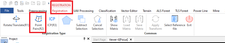
In the toolbar, the “Registration” tab will be highlighted in red, and we will see tools for working with Data Registration. In this case, we are interested in “Point Pairs”, Figure 21. Click on the “Point Pairs” tool.
Figure 21. «Point Pairs» tool.
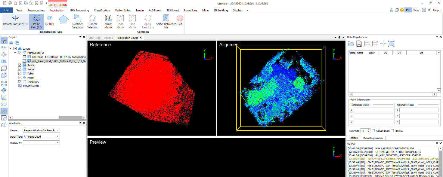
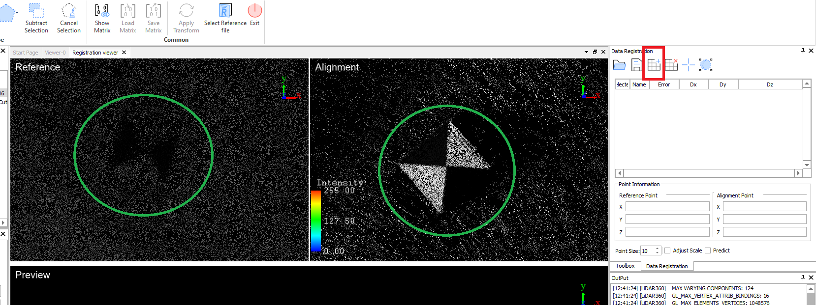
The main working window area will be divided into several parts, Figure 22.
Figure 22. «Point Pairs» workflow.
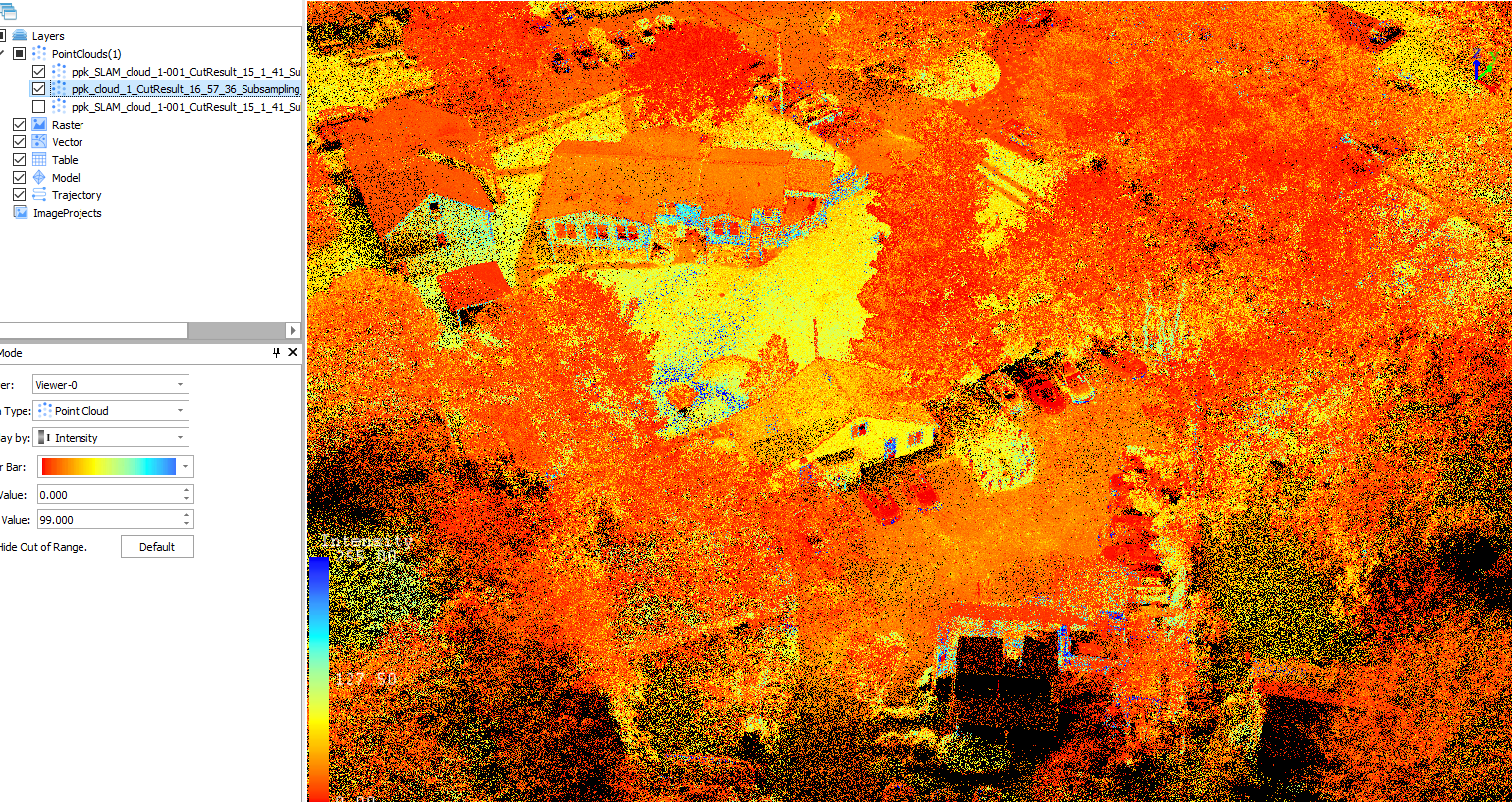
As you can see, the reference cloud is on the left, and the SLAM cloud is on the right.
We recommend displaying intensity using a gray color gradient to improve control point visibility in the clouds. To do this, in the “View Mode” panel, select “Display by” – Intensity. Control points can be any easily recognizable objects, such as special markers, building corners, etc.
After the display has been set up, we move on to searching for objects, Figure 23. When scanning, we used markers, but we will also show that other objects are no worse for georeferencing.
Figure 23. Founded special marker.
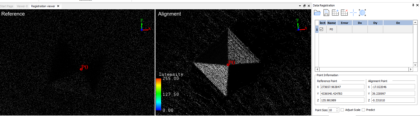
We found a special marker in both clouds, and now we need to add a point. To do this, click “Add Point” in the “Data Registration” panel. The point “P0” will be added to the list of points. Then click “Pick Points” to activate the point selection tool (icon will change the background color to indicate that the tool is active). Click in the reference and SLAM clouds in the same place on the special marker. As a result, the point “P0” will appear in the point clouds, as shown in Figure 24. In order not to accidentally change the point, click on the “Pick Points” to cancel the selection of the tool for adding a point to the cloud.
Figure 24. Set point.
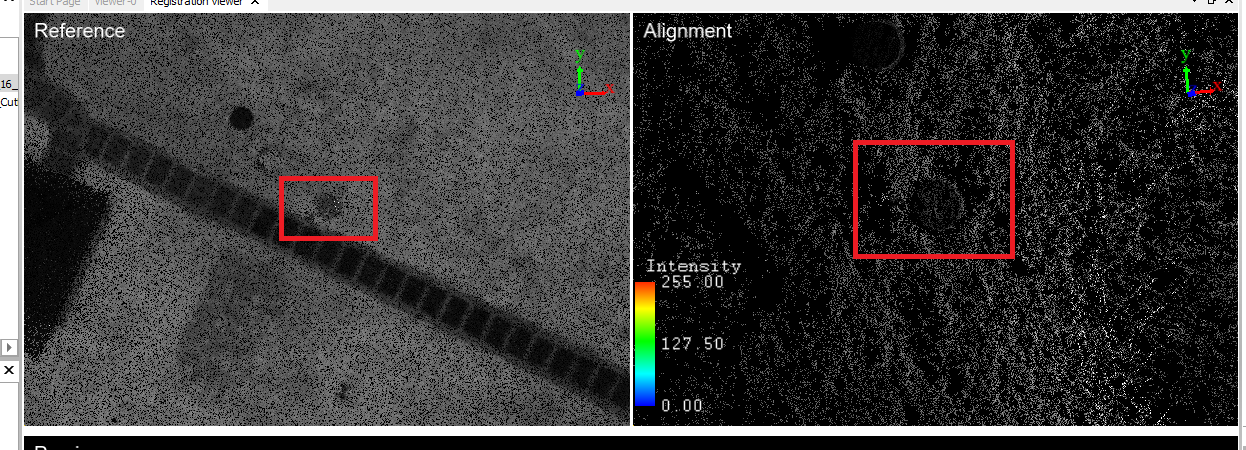
We also look for the next object, which is clearly visible in both point clouds. In our case, it is a round stone, as shown in Figure 25. Also, first, add a new point by clicking on the “Add Point”, and then click on “Pick Points” and add a point to the same place on the point clouds.
Figure 25. Round stone as a control point.
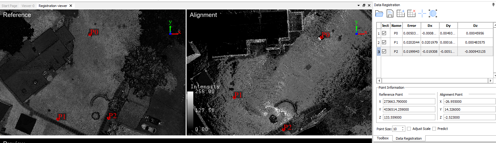
After adding three points—enough for georeferencing—the accuracy calculation results will be displayed, as shown in Figure 26. In our case, we got an accuracy of 2 cm in the horizon Dx, Dy, and less than 1 mm in the vertical Dz. The more accurately the points are selected, the smaller the georeferencing error will be.
Figure 26. The result of calculating the accuracy of the coincidence of points in both clouds.
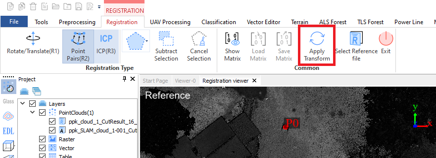
Three points are enough for georeferencing to take into account the slopes in two planes. In this case, the accuracy result suits us. Therefore, the next step is to apply the transformation for georeferencing. Click “Apply Transform” and wait for the process to complete, as shown in Figure 27.
Figure 27. Starting the process of transforming the SLAM point cloud coordinates.
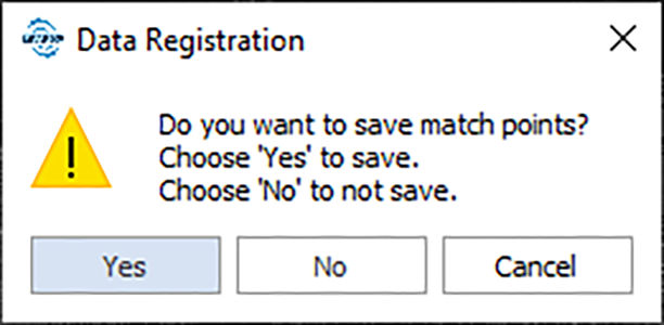
After the process is complete, the program will offer to add data to the project, Figure 28, and save the list of points we selected earlier to a file, Figure 29. Add data to the project and save the list of points. The list of points will be saved in a text file, which is shown in Figure 30.
Our georeferenced SLAM cloud will be displayed in the list of layers. To check, we will use the already familiar “Pick Point” tool, Figure 31.
Figure 28. ToolTip.
Figure 29. Data Registration.
Figure 30. Match-points list.
Figure 31. Checking the georeferencing of the point cloud using the “Pick Point” tool.
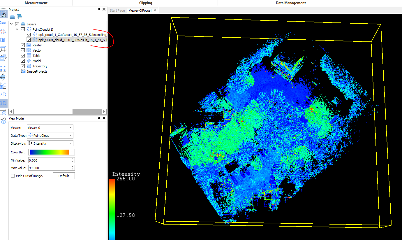
As you can see, this is our SLAM cloud, but already georeferenced. Now we will display only the GNSS cloud, Figure 32. You can see the low density of points in places where the laser beams could not hit during aerial photography.
Figure 32. Only the GNSS cloud is selected.
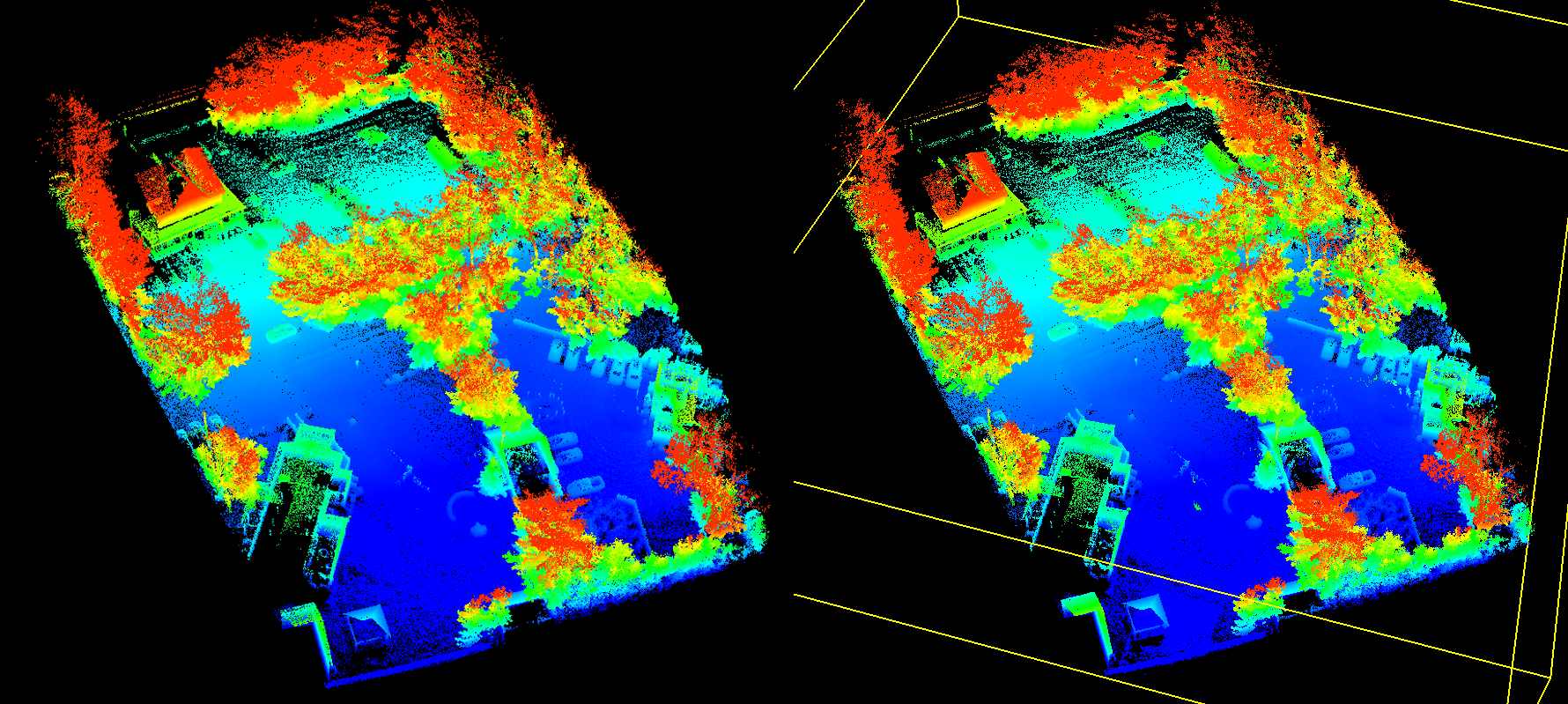
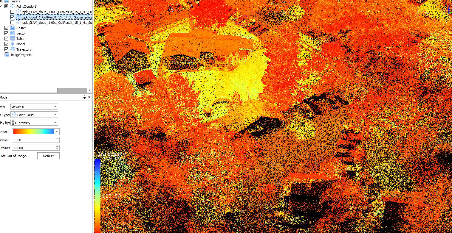
Let’s display both clouds at the same time and look at the result, in Figure 33.
Figure 33. Both point clouds are displayed: GNSS and georeferenced SLAM.
The control point report tool will create a report about the elevation difference between laser point clouds and ground control points, which can be used to check the elevation accuracy of laser point clouds and improve the height accuracy of laser point clouds using calculated adjusted values.
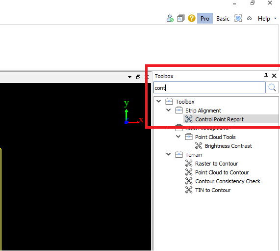
The first report we’ll look at is the “Control Point Report”, which can be found in the “Toolbox” tab.
For a quick search, you can use the search bar by typing the name of the toolbox, Figure 36.
Figure 36. “Control Point Report” in the “Toolbox” tab.
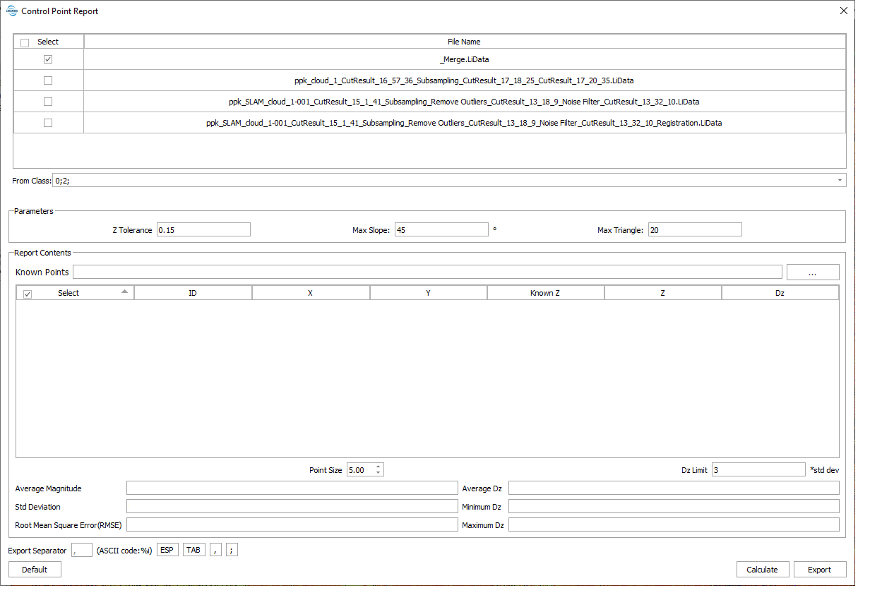
The toolbox is launched by double-clicking on it, after which you will see the window shown in Figure 37.
Figure 37. “Control Point Report” toolbox.
Here it is important to pay attention to the “Report Contents” and the “Average magnitude”, “Std Deviation”, and “Root Mean Square Error (RMSE)” display fields. They will display information about the accuracy of the point cloud.
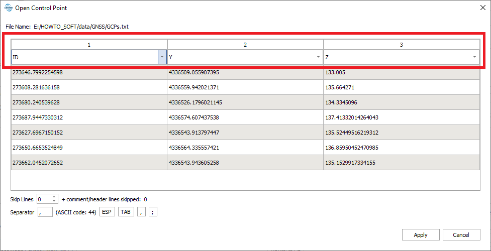
To load checkpoints, click on the button with three dots next to the “Known Points” field. A window, shown in Figure 38, opens.
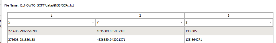
If necessary, you can change the type of column according to the data. By default, the first column is assigned as the point number. In our case, it is not in the text file, so we replace the first column in the drop-down list with “X”, the second and third will be the coordinates “Y” and “Z”, respectively, Figure 39.
Figure 38. “Open Control Point” window.
Figure 39. Correct loading of checkpoints.
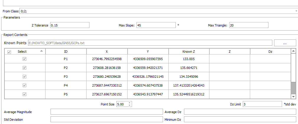
After the setup, click on “Apply”. The Open Control Point window closes and we see a list of control points in the Control Point Report window, Figure 40.
Figure 40. A list of checkpoints.
In this case, we will leave the parameters by default. We will only note that:
Z tolerance (default value is “0.15”): The accuracy of the point cloud in the Z-axis direction. To avoid the distance between the points being too small leads to an excessive slope.
Dz limit (default value is “3”): Set the tolerance of Dz. If Dz is not within the tolerance, show red in order to inspect the elevation difference with a large error between the point cloud and control points. Maximum tolerance = Average Dz + Dz * Std Deviation. Minimum tolerance = Average Dz – Dz * Std Deviation
To start the calculation, click on the “Calculate” button in the lower right corner of the window.
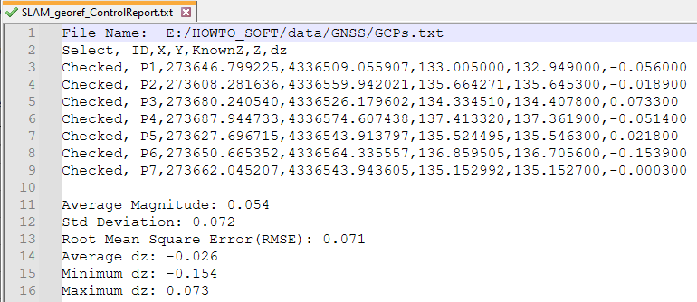
The result is a report on the accuracy of our scan, Figure 41.
Figure 41. Point cloud Z-accuracy report.
To export the report to a file, click on “Export”. A save window will open, where you specify the path where you want to save the report. The report will contain information about the control points and the results of the calculated accuracy, as shown in Figure 42.