For beginners of LiDAR payloads, geolocating SLAM data can be a big challenge. But it’s actually very simple. This guide will show how to georeference SLAM point cloud data from RESEPI in CloudCompare. We will also look at how to generate reports and show you the key aspects to pay attention to.
Any activity with point clouds begins with the import of data. In LiDAR360, this can be done in several ways:
Use the Quick Access menu in the upper-left corner, as shown in Figure 1.
Click on the “File” button, and then click on “Open”.
This will open a window where you need to specify the path to the .las (.laz) file.
Figure 1. Import data.
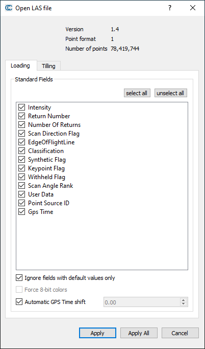
A window with import parameters will appear, as shown in Figure 2. Just click “Apply”.
Figure 2. Import Parameters.
A window with scaling settings will appear, as shown in Figure 3. Click “Yes”.
Figure 3. Scaling Parameters.
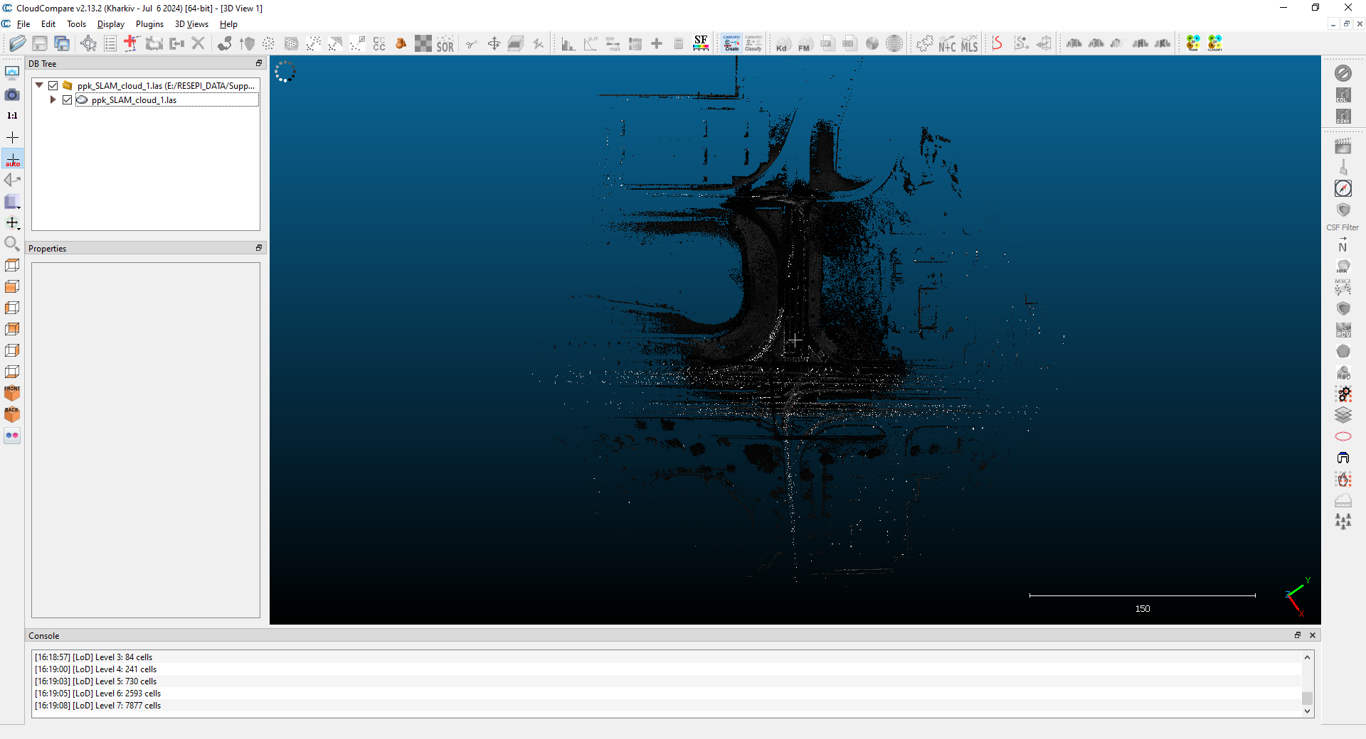
As a result, our point cloud will be displayed in the main window, as you can see in Figure 4.
Figure 4. Point Cloud in the Viewing Window.
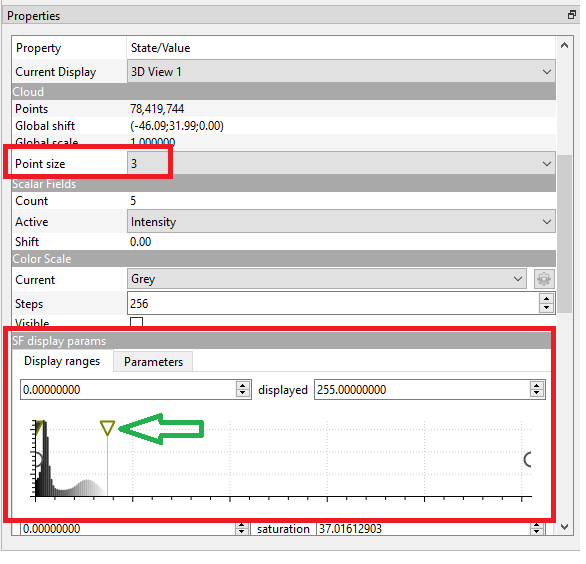
Click on the point cloud file to display its properties in the “Properties” tab, as shown in Figure 5.
Figure 5. Point Cloud Properties.
Change the point size using the dropdown list “Point size”.
In the “SF Display params” tab, adjust the intensity display using the slider with the triangle, as shown in Figure 6. This will change the intensity of the coloring.
Click on the alignment tool “Align” in the Quick Access Panel, as shown in Figure 7. It is also available in the main upper toolbar or under the “Tools > Registration > Align (point pairs picking)” menu.
Figure 7. Alignment Tool.
A window, as shown in Figure 8, will appear. It will display the control points and the points that we select on the point cloud.
Figure 8. "Align" Tool Window.
Click on the place in the point cloud where the GCP will be attached. In this case, it is the tip of the road marking arrow, as shown in Figure 9. The coordinates of the selected point will be displayed in the list of points to be georeferenced.
Figure 9. Adding a Point to the List.
Click the pencil icon to add a GCP, as shown in Figure 10. A window will appear where you need to enter the GCP coordinates.
Figure 10. Adding GCP.
Do the same to add two more points. As a result, the list of points will look as shown in Figure 11. Click on “Align”.
Figure 11. Adding 3 Control Points.
The point cloud will align with the control points, and now we can fine-tune the result to achieve even greater accuracy. To do this, zoom in to the first control point “A0”, as shown in Figure 12. You will notice that our manually added point “A0” is located some distance from the reference “R0”. In addition, another point is located much closer to “R0”.
Figure 12. The First Reference Point "R0".
Therefore, the next step is to more precisely position the points that need to be tied to the GCPs. To do this, delete the manually added points by clicking on the clear icon, as shown in Figure 13.
Figure 13. Deleting Added Points.
After deletion, click on the point that is closest to the GCP, as shown in Figure 14. Repeat the procedure for the remaining points. We also emphasize the fact that the points should be corrected in the same order as they appear in the list, i.e., first, adjust the pair “A0-R0”, then “A2-R2”, etc.
Figure 14. Adjusting the Coordinates of the First Point "A0".
As a result, more precise georeferencing is achieved. The result is shown in Figure 15.
Figure 15. Adjustment Result.
Click on the green check mark to apply the changes. The window shown in Figure 16 will open. It shows the resulting transformation matrix and scaling factor. Click “OK”.
Figure 16. "Align info" window.
The window shown in Figure 17 will open. Click “Yes”.
Figure 17. Scaling Parameters.
As a result, we obtained a geo-referenced SLAM point cloud with an error of less than 2 cm, as shown in Figure 18.
Figure 18. The result of georeferencing the SLAM point cloud.