Contour lines, the Digital Elevation Model (DEM), and the Digital Surface Model (DSM) are commonly used geospatial deliverables derived from point clouds. This guide will show how to retrieve these models from a point cloud from RESEPI in TerraScan, and TerraModeler by Terrasolid. In this case, the Microstation platform from Bentley Systems Inc. was used, but this tutorial will be useful when using the Spatix platform as well. We will also look at how to generate reports and highlight the key aspects to consider.
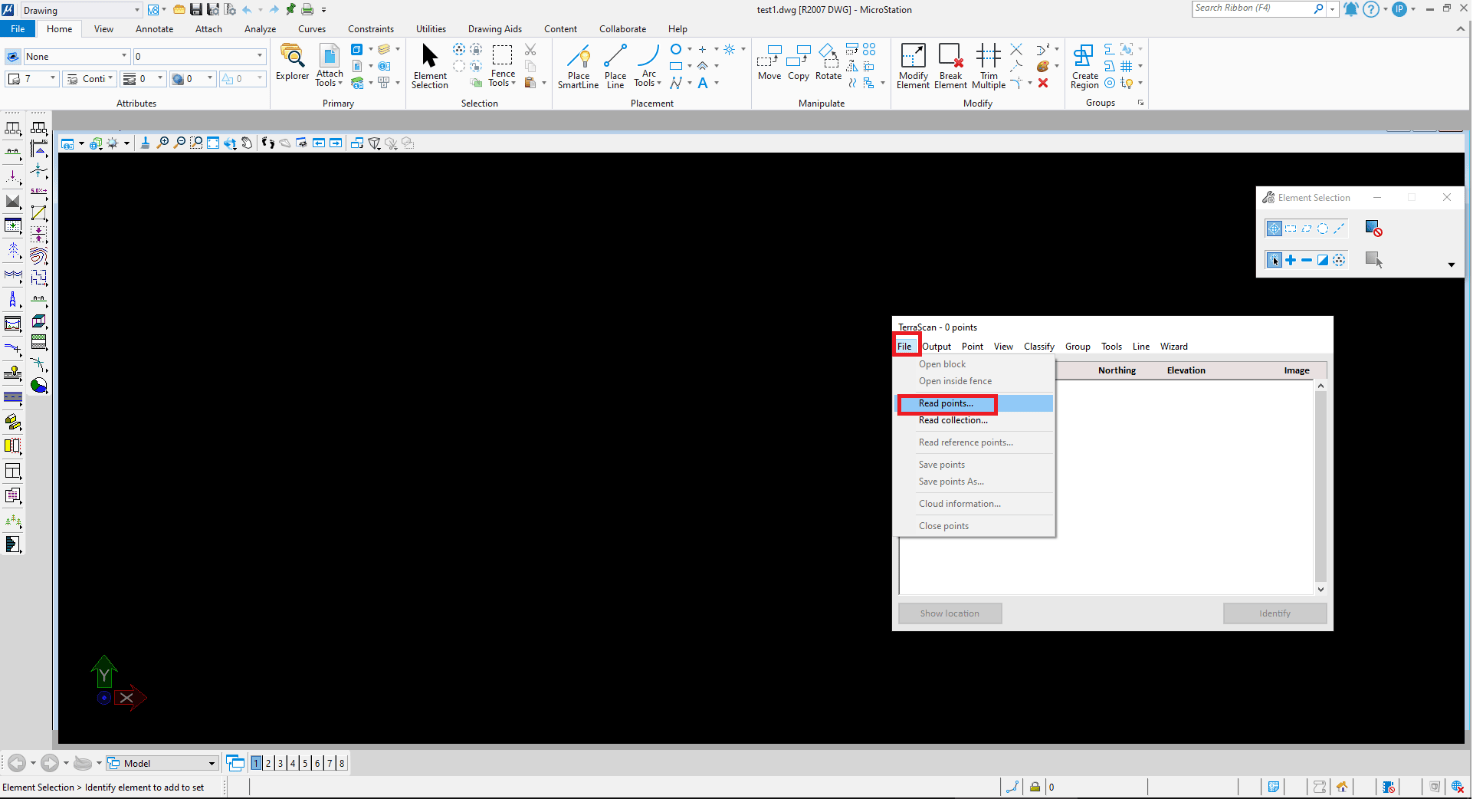
Any work with point clouds begins with importing data. To import the data, click on “File” -> “Read points…” in the menu, as shown in Figure 1.
Figure 1. Open data file.
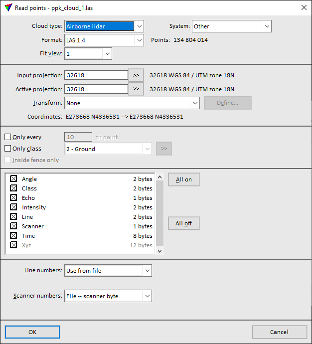
This will open a window for selecting the path to the point cloud location. Select the desired point cloud and click “Open”. After that, the window shown in Figure 2 will open. As you can see, the program automatically detects the projection (default UTM for RESEPI data) and the zone number. Here it is important to choose the correct type of point cloud, as this is recommended to optimize the processing speed for many automatic procedures. In this case, we will process aerial data that were recorded by a mobile lidar, so we select “Airborne Lidar” in the drop-down list. Let’s leave the other parameters unchanged and click on “OK”.
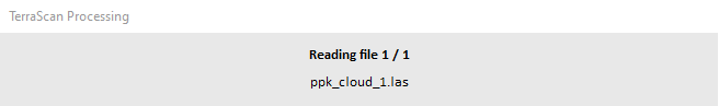
The import process will start, and it may take some time. During the process, the window shown in Figure 3 will be displayed, demonstrating that the point cloud is being loaded for further work.
Figure 2. Data import parameters.
Figure 3. Point cloud loading process.
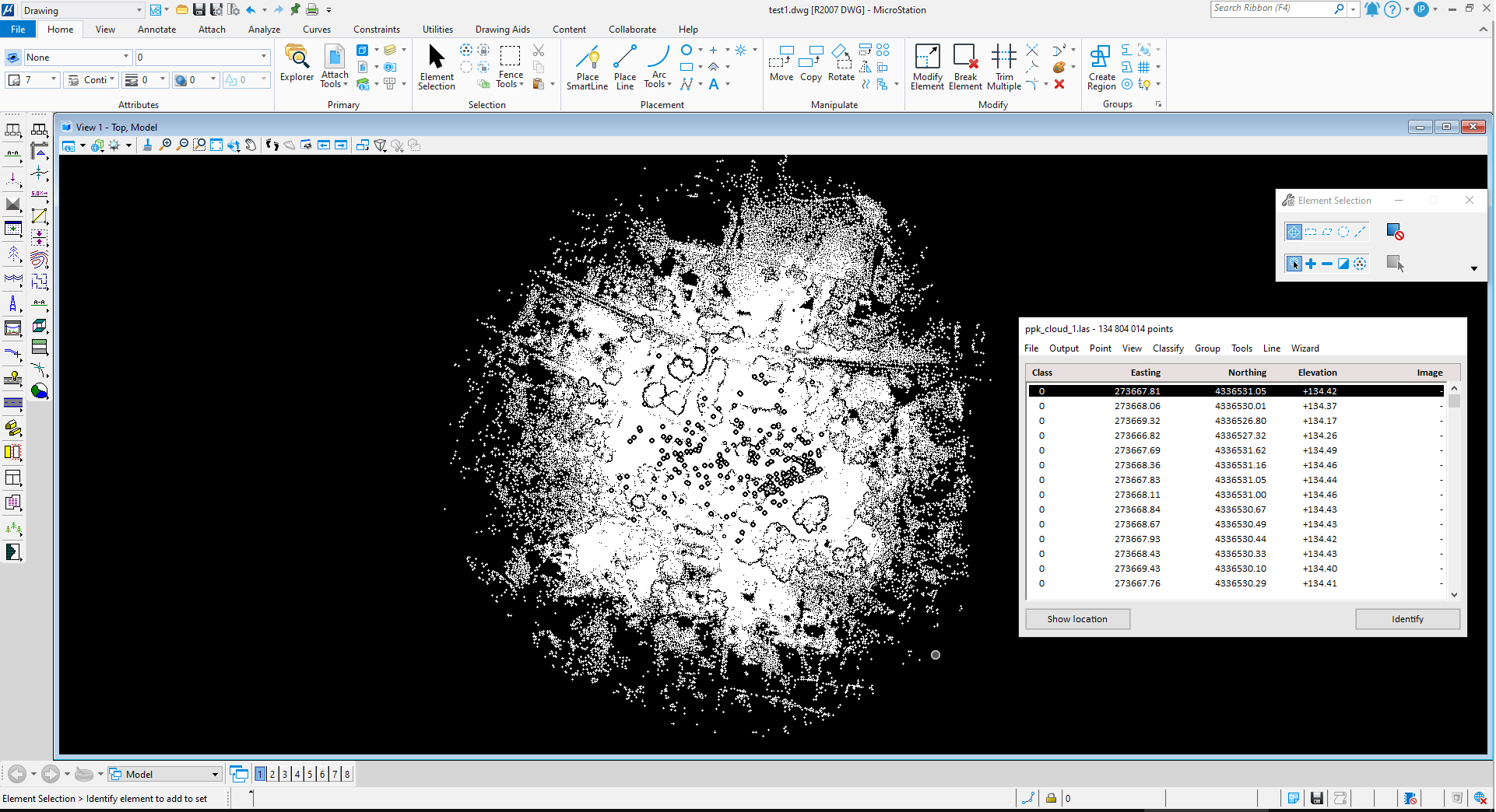
Once the loading process is complete, the main program window will look as shown in Figure 4. As you can see, the Terrascan window automatically displays a list of points where you can find out the coordinates of the point and the class it belongs to. By default, all points are unclassified and belong to the general class “Class 0”.
Figure 4. The main window of the program after loading the point cloud.
For further work, we will need to familiarize ourselves with the classification procedure, but first, let’s cut off the unnecessary areas in our point cloud. To do this we need to:
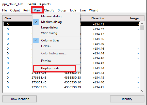
Click in the menu “View” -> “Display mode” and change the color of the unclassified cloud to something other than white, Figure 5.
Figure 5. Display options.
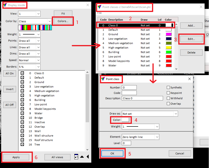
This will open the “Display mode” window where we click on “Colors” 1, Figure 6.
This will open the ‘Point Classes’ window, where you can select the class whose color you want to change 2 and click “Edit” 3.
The window “Point class” opens in which you click on the color next to the field “Color” 4 and change it, for example, to gray. After changing the color, click on “OK” in the “Point Class” window. This will close it.
Click on “Apply” in the “Display mode” window and the point cloud will be colored as shown in Figure 7.
Figure 6. Changing the color of an unclassified point cloud.
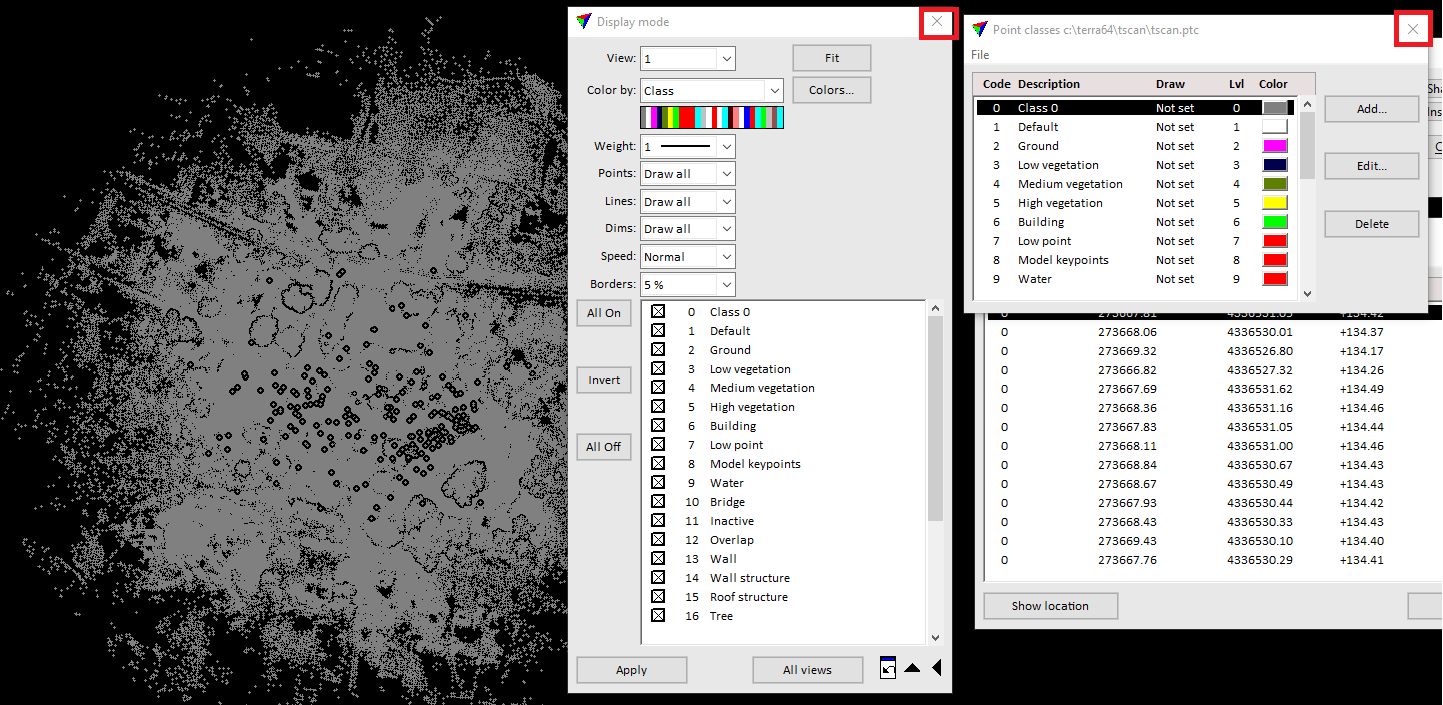
The windows can then be closed by clicking on the cross in the upper left corner, Figure 7.
Figure 7. Changed color for the unclassified point cloud.
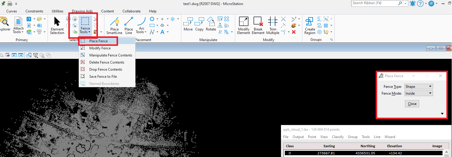
Now we can remove unnecessary points using the “Fence Tools”, which is located in the toolbar, Figure 8.
Click on “Fence Tools” in the toolbar and select “Place Fence”.
A window will appear on the right with options for selecting the area. For convenience, select the same options as shown in Figure 8. This allows us to select arbitrary polygonal areas for deletion instead of just rectangular ones (the default setting).
Figure 8. Cut tool.
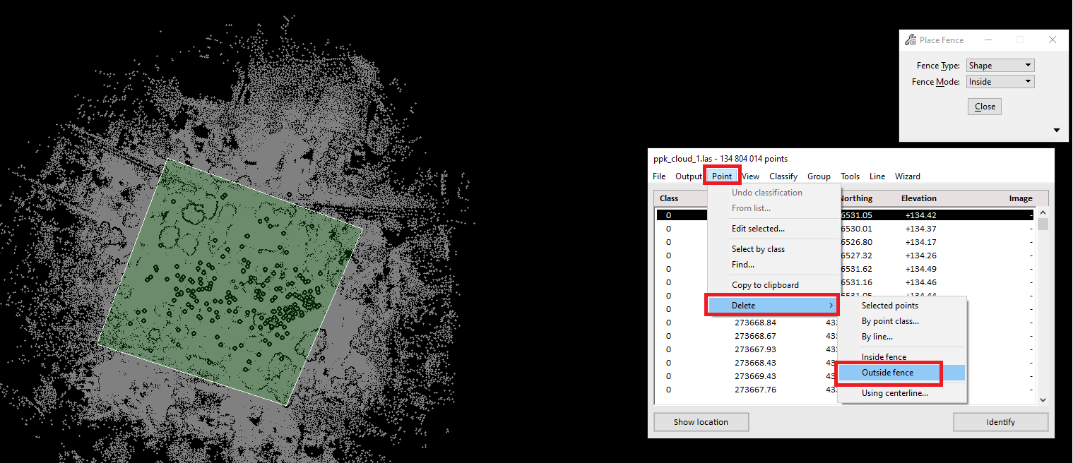
Select the desired area and click on “Point” -> “Delete” -> “Outside fence” as shown in Figure 9.
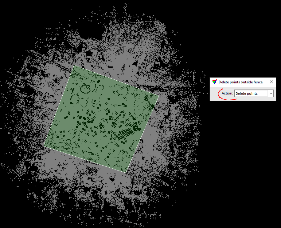
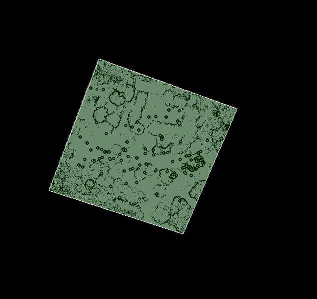
The “Delete points outside fence” window will open, Figure 10. Then click anywhere on the point cloud to accept the changes. As a result, the points that are located “outside” the selection area will be deleted, Figure 11.
Figure 9. Menu for deleting points outside the selection area.
Figure 10. Deleting points.
Figure 11. Points outside the selection area are deleted.
As you may have noticed, the lines that are displayed for the selection area are white. Since the point cloud is unclassified by default and is also white, the lines would not be visible when defining the area. So, we immediately changed the color of the cloud for ease of operation.
Now we will prepare the point cloud for DSM/DEM generation and the first step is to remove unnecessary points and noise. To do this, we will display the cloud from the side view. For this purpose, it is necessary to:
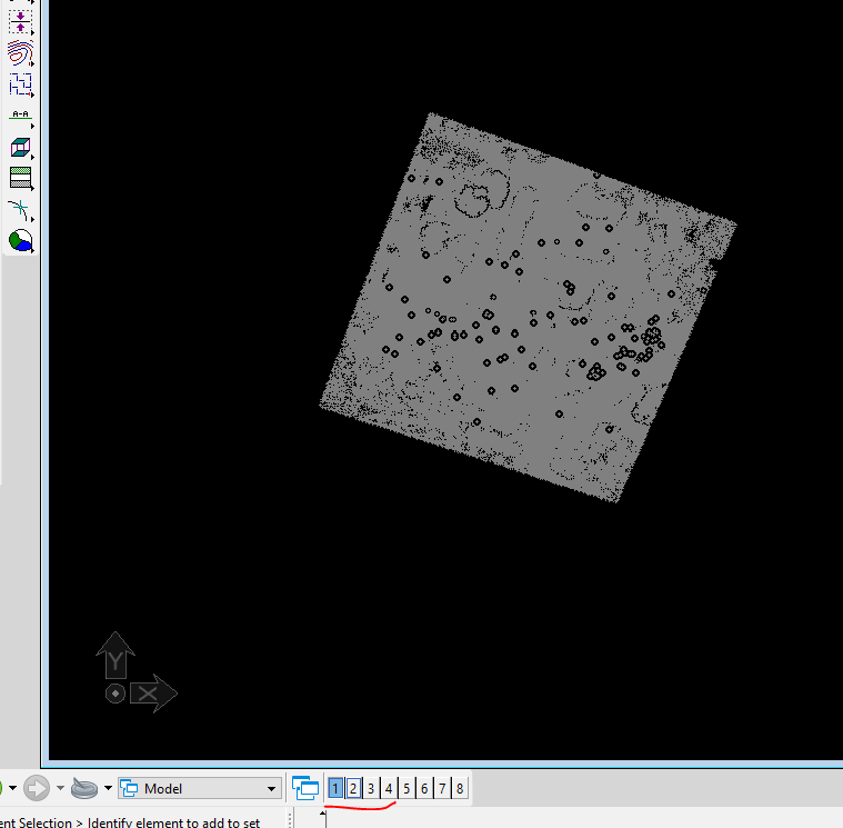
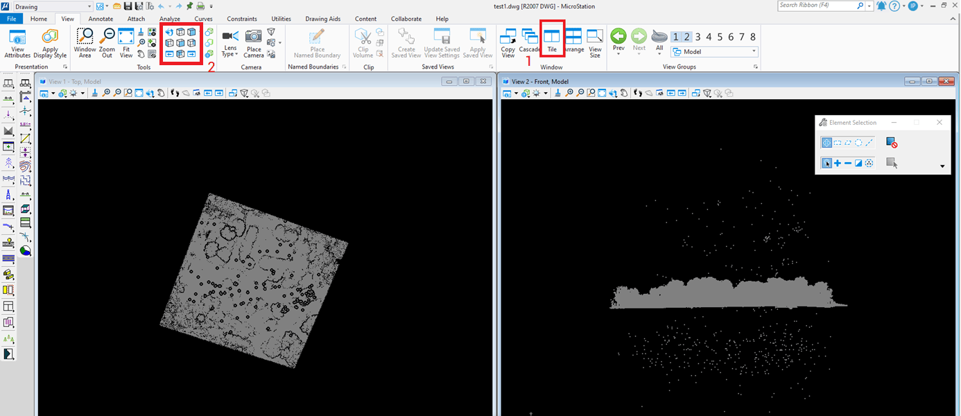
Add another view window by clicking on “2” in the “View Toggles” menu, as shown in Figure 12.
Figure 12. "View Toggles" menu.
Click on “Tile” 1 to place the windows side by side. Then click on “View 2” to make it active, and change the view to “Right View” 2, as shown in Figure 13. As you can see there is a lot of noise in the point cloud that needs to be removed.
Figure 13. Arrangement of the two view windows.
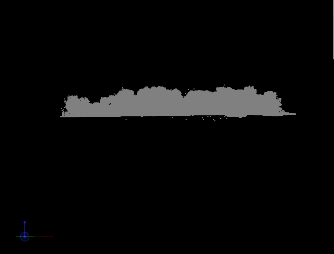
To remove the noise, we can use the same tool we used earlier (“Fence Tools”) or we can use classification to automatically detect the noise. In this case, we will use both tools. For rough cleaning we will use “Fence Tools”, but now we will delete points that are inside the selection area: “Point” -> “Delete” -> “Inside fence”. As a result, the point cloud will look as shown in Figure 14.
Figure 14. The point cloud after rough cleaning with “Fence Tools”.
As you can see, most of the noise has been removed, but not completely, so we move on to classification for better cleaning.
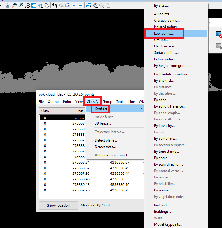
In the menu “Classify” -> “Routine” selects the desired type of classification. First, we will remove the points that are below the surface level. To do this, click on “Low points…”, Figure 15.
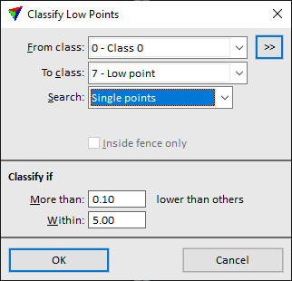
A window with classification parameters will open, as shown in Figure 16. In this window, you need to adjust the parameters, as they are essential for accurate classification.
Select the desired class “Class 0” from the drop-down list. The program has automatically selected the class to which the points “7 – Low Point” will be assigned.
In this case we will search for single points that are farther than 0.1 m from the other points, so change the parameter next to the “More than:” field to 0.1 meters. Click “OK”.
Figure 15. Classification menu.
Figure 16. Classification parameters for "Low Points".
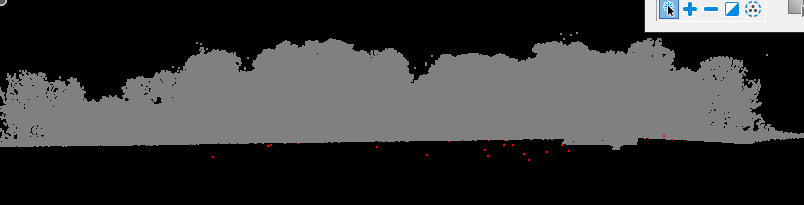
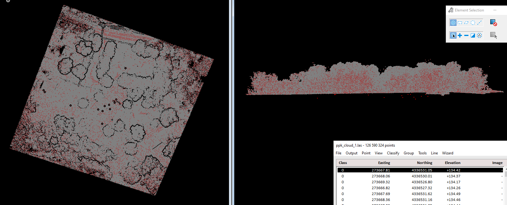
As a result, the noise that is “under the cloud” is classified as a “Low point”. The program automatically highlighted them in red for better visibility, as shown in Figure 17.
Figure 17. The noise is classified as a “Low Point”.
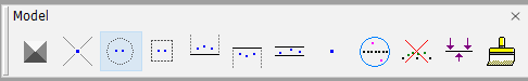
If after the “Low point” classification in automatic mode there are points that can also be classified as “Low point”, but they were not determined by the program (this is due to the parameters), then they can be conveniently and quickly deleted manually. To do this, you will need the toolbox, which is available from the menu “Tools” -> “Toolboxes” -> “Model” in the Terrascan window. The appearance of the toolbox toolbar is shown in Figure 18.
Figure 18. Appearance of the "Model" toolbox toolbar.
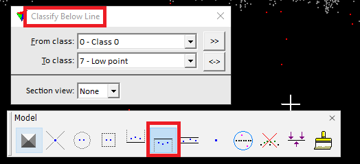
Click on the icon shown in Figure 19 to select the “Classify Below Line” tool. In the window that opens, select the class whose points will be placed in “Low Points”.
Figure 19. Selecting the "Classify Below Line" tool and setting the classification parameters.
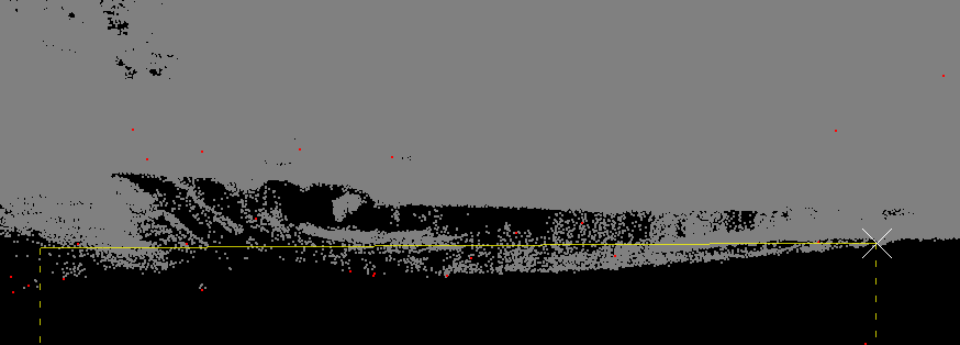
After that, draw a line over the points that we want to classify, as shown in Figure 20. Click in the desired place in the point cloud to confirm the operation.
The points under the line will be classified as “Low Points”, as indicated by the color of their selection, as shown in Figure 21.
Figure 20. Manual selection of points for classification as "Low Points".
Figure 21. The points under the line are colored red, according to the color of the "Low Points" class.
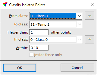
In the same way, we classify “Isolated Points” with the parameters that are shown in Figure 22. The result of the classification is shown in Figure 23.
Figure 22. Classification parameters for "Isolated Points".
Remember that for your dataset the suitable parameters may be different!
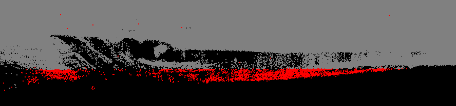
Figure 23. Classified “Isolated Points”.
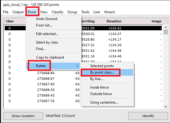
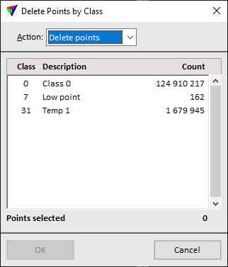
Now we will delete these points using the menu “Point” -> “Delete” -> “By point class…” as shown in Figure 24.
A window will open with the existing point classes, Figure 25. Select “Low point” and click on “OK”. The selected points will be deleted.
Repeat the procedure for the “Temp 1” class.
Figure 24. Point class deletion menu.
Figure 25. Selecting the class to be deleted.
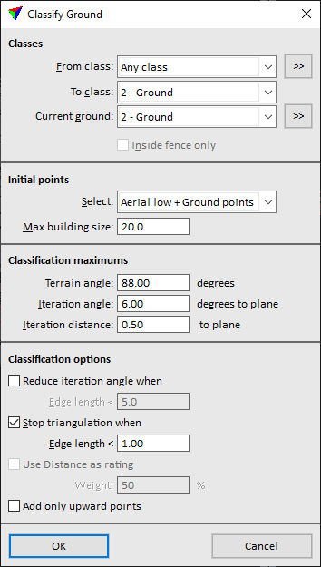
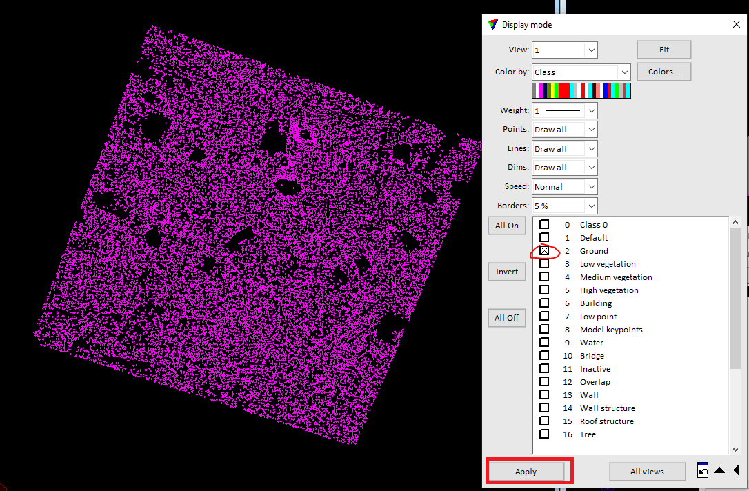
After cleaning you should classify the surface points, called “Ground” points. We used the parameters shown in Figure 26. The result of the classification is shown in Figure 27. For this display, you should go to “View” -> “Display mode” and leave a checkmark on the class you want to keep for display, then click on “Apply”.
Figure 26. Parameters for “Ground” classification.
Figure 27. The result of “Ground” classification.
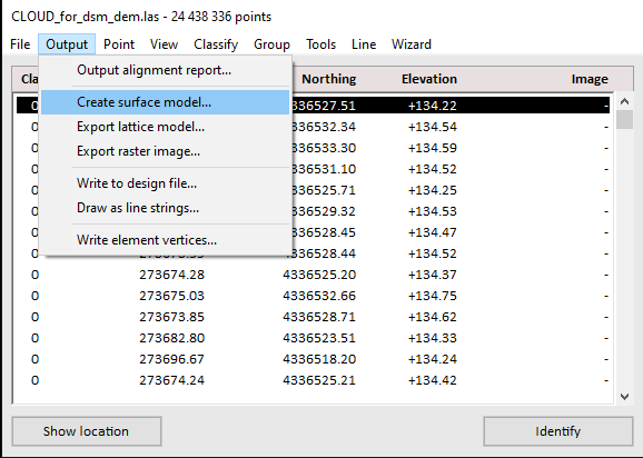
Since we are satisfied with the result, we can proceed with DSM/DEM generation. Point Cloud to Digital Elevation Model and Digital Surface Model To generate a DEM, follow these steps:
Click on the menu “Output” -> “Create surface model…”, Figure 28.
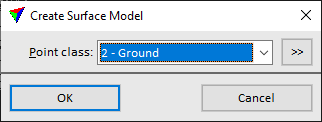
In the window that opens, as shown in Figure 29, select the class and click “OK”.
Figure 28. Export menu.
Figure 29. Class selection.
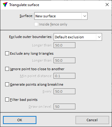
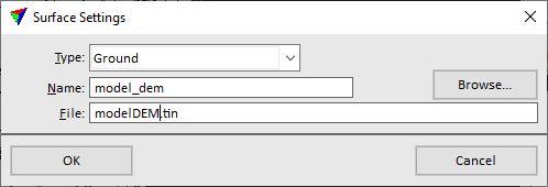
The surface creation settings window will open, as shown in Figure 30. Select the parameters and click “OK”. A window opens to select the file path, name, and model type. Select the type “Ground” and enter a name, then click “OK” as shown in Figure 31.
Figure 30. Parameters window for creating a surface.
Figure 31. Selecting the surface type, model name, and file saving path.
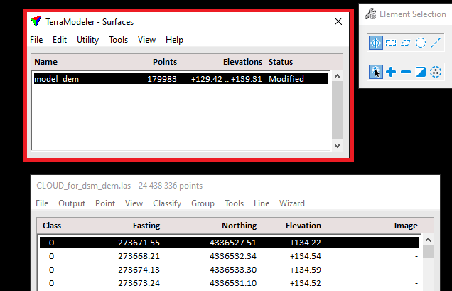
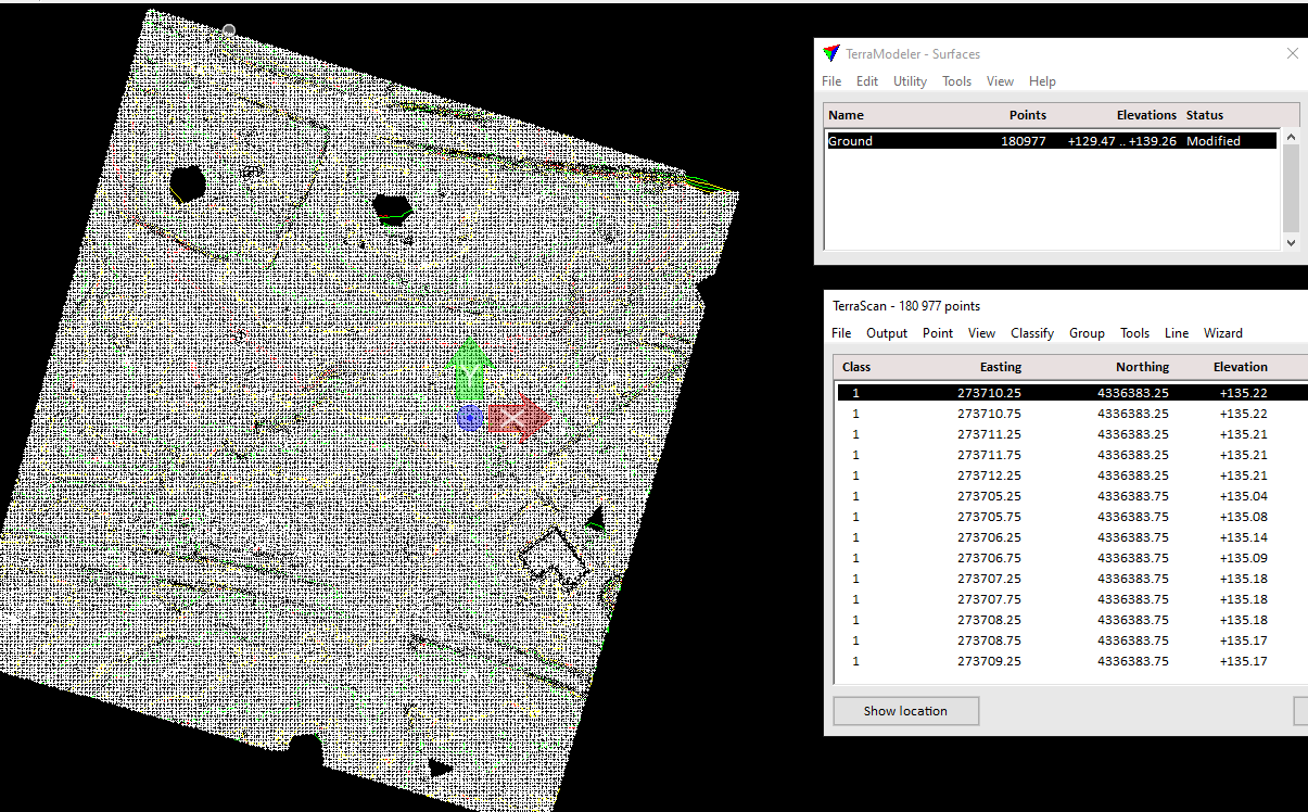
The created model will then be displayed in the list of models in the TerraModeler window, as shown in Figure 32.
Figure 32. The created model is displayed in the model list.
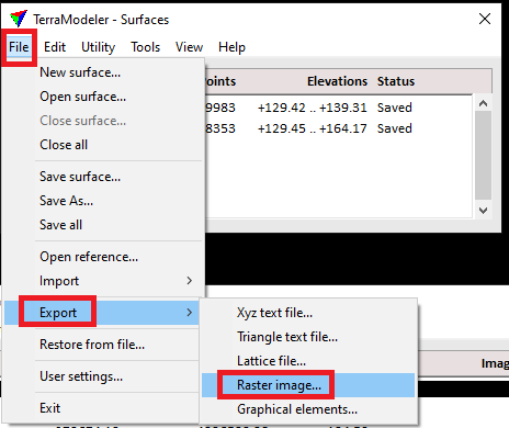
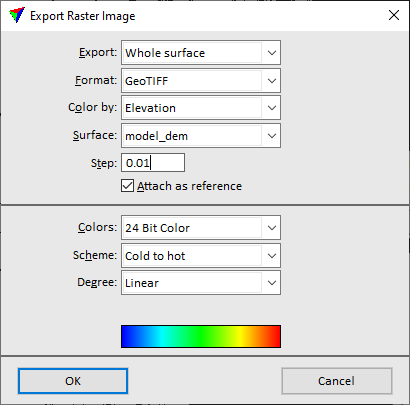
In the “TerraModeler” window in the “File” menu click on “Export” -> “Raster image”, Figure 33. The window shown in Figure 34 will open. In this window, you can customize the export parameters. We will export to GeoTIFF with a grid spacing of 0.01. The rest of the parameters we leave by default.
Figure 33. Model export.
Figure 34. Export parameters.
In the opened window specify the path where we want to save the GeoTIFF file.
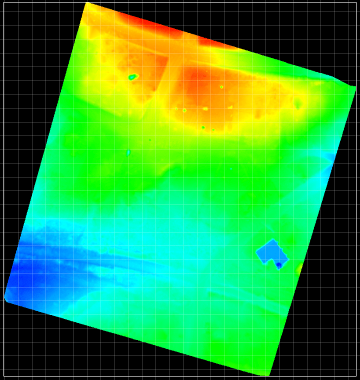
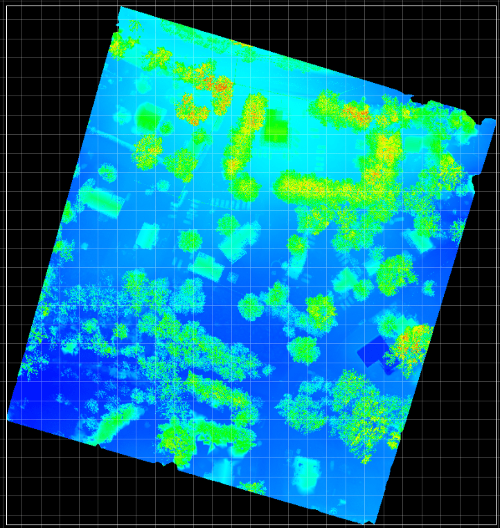
The same procedure will be used to obtain DSM, but “Any Class” is selected when selecting the class of points for model creation. Therefore, we will not dwell on this in detail but just demonstrate the result, in Figure 35, and Figure 36.
Figure 35. DEM.
Figure 36. DSM.
Now we will proceed to the generation of contours.
We will use our point cloud, which already has “Ground” point classification, to generate the contours. Now we will export these points to a text file. To do this you need to:
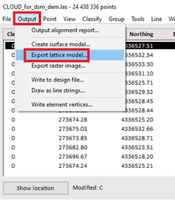
Click on “Output” -> “Export lattice model…” as shown in Figure 37.
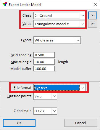
The window shown in Figure 38 will open. Here we have to make sure that the class “Ground”, “Triangulated model z” and the file format “Xyz text” are selected.
Figure 37. Lattice model export menu.
Figure 38. Export parameters.
A window will open in which you should specify the path and the name of the file to be saved, we called it “ground_points.xyz”.
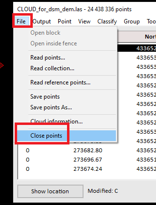
Close the current point cloud by clicking on “File” -> “Close points” as shown in Figure 39.
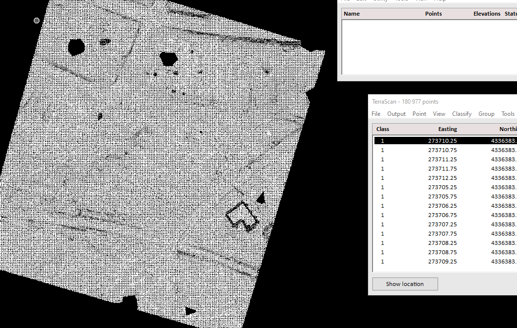
Then open our file with saved ground points “ground_points.xyz”. In our case, the result is shown in Figure 40.
Figure 39. Closing the point cloud.
Figure 40. Visualization of points from the file “ground_points.xyz”.
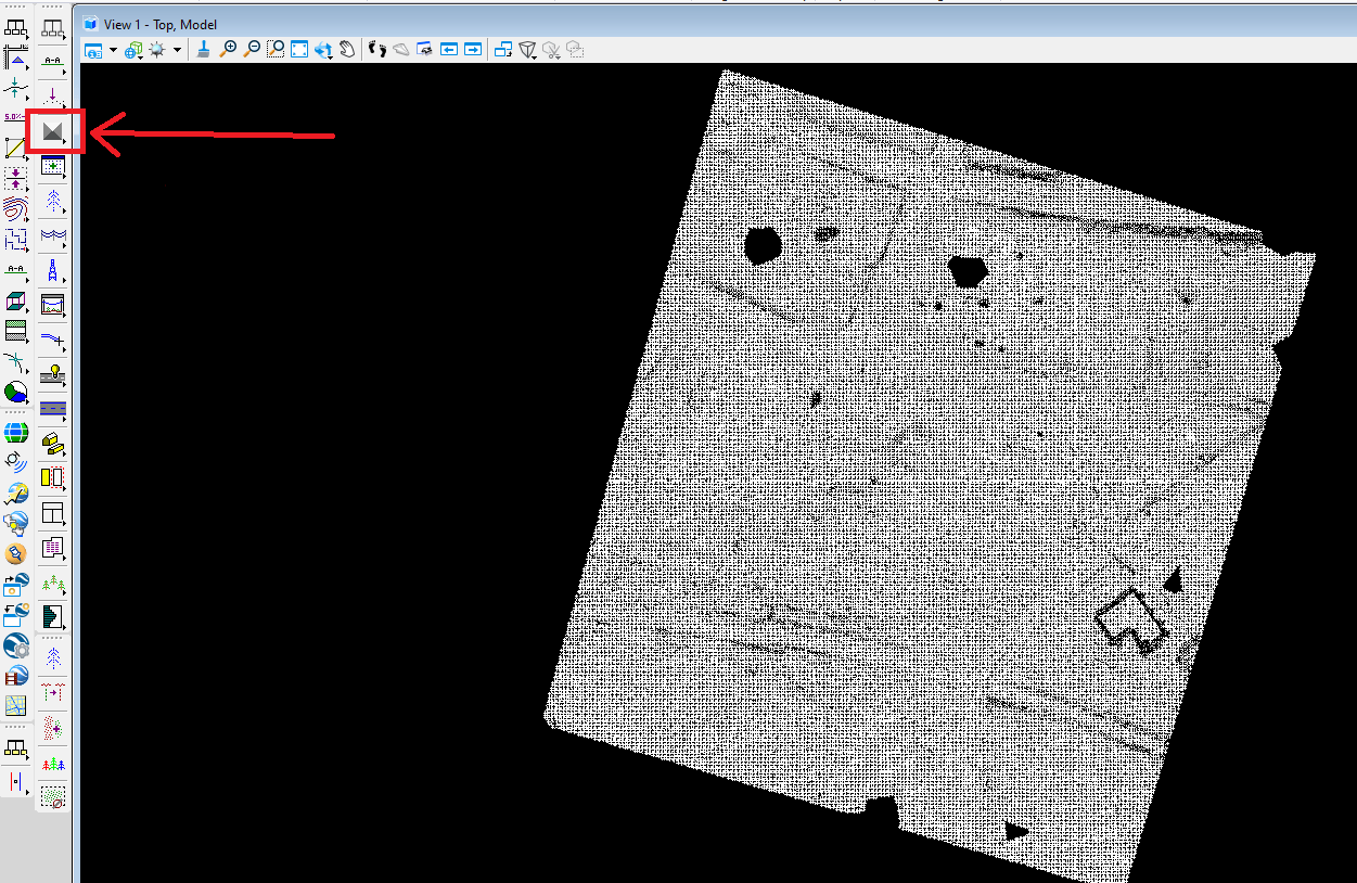
Now we will create a model based on the loaded points. To do this, click on the icon shown in Figure 41.
Figure 41. Starting the model builder.
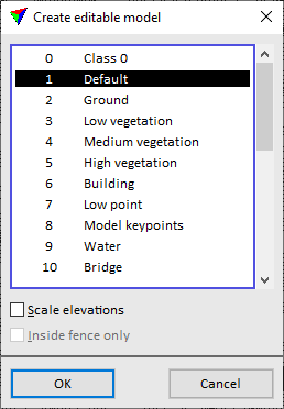
The window shown in Figure 42 will open. Here we specify “1 Default” because in this case our points have been automatically assigned to this class, unlike the point cloud which had “class 0” by default. Click on “OK”.
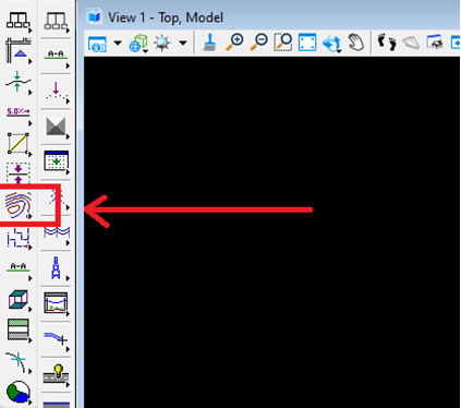
After that our model has been successfully created and we will generate contours from it. To do this, click on the icon shown in Figure 43.
Figure 42. Selecting a class for the model.
Figure 43. Selecting a tool for drawing contours.
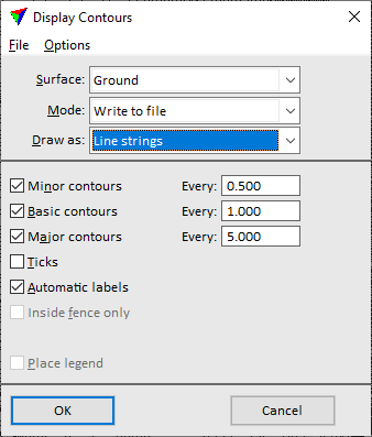
The window shown in Figure 44 will open. We will save our contours to a file by selecting the “Write to file” mode and enabling “Line Strings” rendering. Leave the other parameters unchanged. Click “OK”.
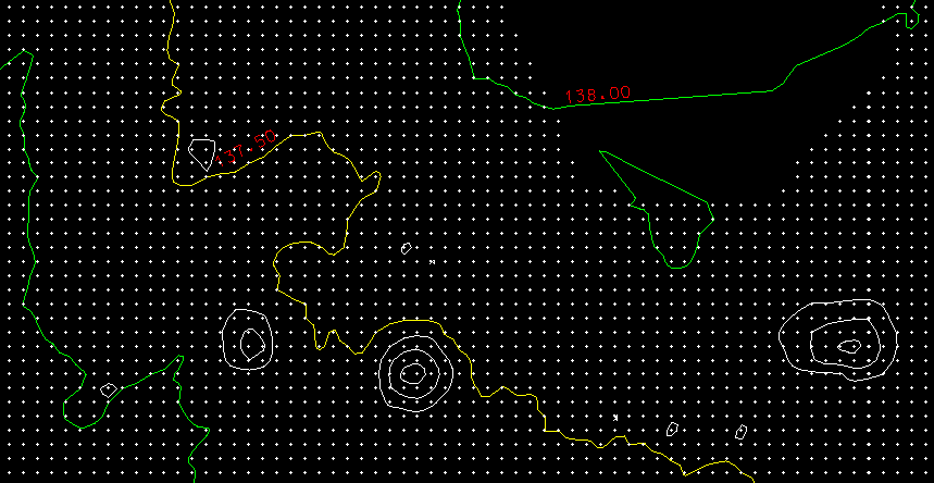
After data processing in the program window, we will see the contour and the model in the list of models, Figure 45. To explore the surface, increase the zoom, Figure 46.
Figure 44. Parameters of contour creation.
Figure 45. Created contours.
Figure 46. Contours when zoomed in.
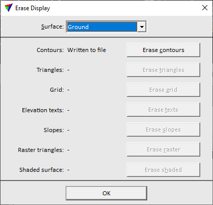
vTo remove the contours from viewer window, click on a tool for drawing contours and click on “Erase Display” tool. The window shown in Figure 47 will open. Click on “Erase contours” and click “OK”. After this, the contours will be removed from the viewing window.
Figure 47. "Erase Display" window.
We will now look at the process of obtaining accuracy reports for our point cloud and DSM/DEM models using GCPs.
The Control point report tool outputs an accuracy report between the point cloud and the independently surveyed control points and checkpoints. These values can then also be used to manually register the point cloud to the desired altitude values.
To get an accuracy report you need to:
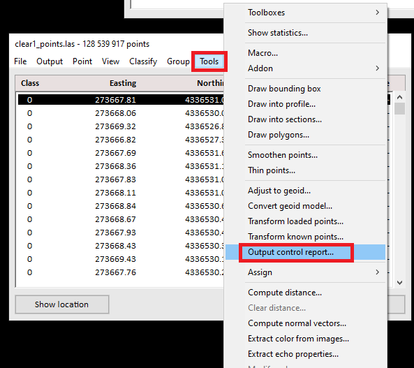
Click on “Tools” -> “Output control report…” menu, Figure 48.
Figure 48. Create a height accuracy report.
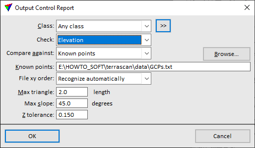
The window shown in Figure 49 will open. Here you can enter the path to the file with the control points, select the class, the type of control (in this case height is selected), and the parameters to be calculated (we left them unchanged). Click “OK”.
Figure 49. Accuracy estimation parameters.
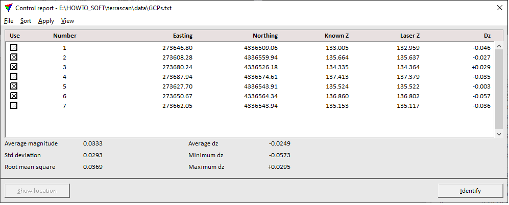
Once the accuracy has been calculated, the window shown in Figure 50 will open. The window will show the control points and the difference between the point cloud and the control point. At the bottom of the window, you will see the average accuracy, the minimum and maximum values, as well as the STD, and RMS.
Figure 50. Height accuracy report by control points.
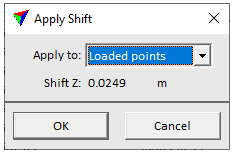
To immediately apply the calculated shift to the point cloud, click “Apply” -> “Elevation shift…” in the menu. The window shown in Figure 51 will open, where you can select which points the shift will be applied to. We will apply the shift to all loaded points, so click “OK”.
Figure 51. "Apply Shift" parameters.
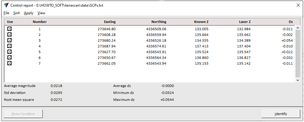
After this, the shift will be applied to the entire point cloud, and the values in the “Control report” window will change taking into account the shift. The result of the operation is shown in Figure 52.
Figure 52. As a result of the height correction, the average error value = 0.
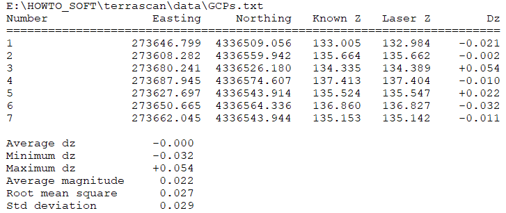
This information can be saved as a text file. To do this in the “Control report” window click on “File” -> “Save as text…”. Then in the opened window select the path where the report will be saved. If you open the report for viewing, it will look as shown in Figure 53. The content of the text file completely duplicates the content of the “Control report” window.
Figure 53. Viewing the report.
The saved report can be easily distributed to clients.
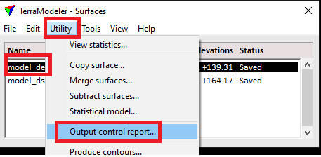
To get the DSM/DEM accuracy report, select the desired model and go to the menu “Utility” -> “Output control report…” as shown in Figure 54.
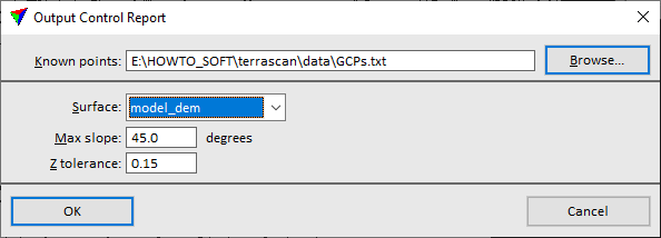
A window will open as shown in Figure 55, where you set the path to the file with control points, as well as the accuracy thresholds for the validity of the points. After selecting the file and setting the parameters, click on “OK”.
Figure 54. Menu section to generate the report.
Figure 55. Setting the parameters for the report generation.
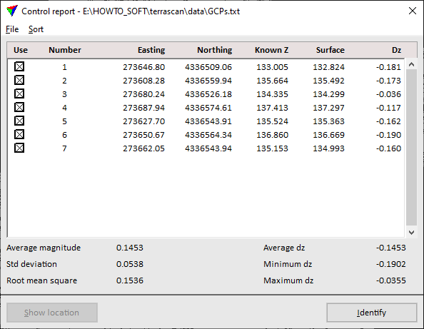
This will open the familiar window with the accuracy information for each control point, Figure 56. As for the point cloud, this information can be saved to a text file for later use. To do this, click on “File” -> “Save as text…”.
Figure 56. DEM Accuracy Report.
The report for the DSM is generated in the same way.