
RESEPI Application Suite User Guide #
1. Introduction & Overview #
The RESEPI Application Suite is a comprehensive toolkit designed for professionals working with LiDAR data acquisition, system testing, and post-processing. The suite centralizes various utilities into a single interface, allowing users to plan missions, diagnose hardware data, simulate communication protocols, and process imagery efficiently.
The suite is divided into several key modules accessible via the main dropdown menu at the top of the application window:
Mission Planner: A calculator for determining optimal flight parameters based on desired LiDAR output metrics.
LiDAR Scan Diagnostics: A tool for analyzing raw .scan files to check for data integrity and hardware performance.
MavLink Simulator: A utility for simulating MavLink data streams to test Ground Control Station (GCS) communication without actual hardware.
Image Processing: A collection of tools for manipulating imagery, specifically focusing on geotagging (GPS EXIF writing).
System Diagnostics (RESEPI LITE & RESEPI GEN-II): Modules for analyzing system logs to generate reports and identify potential issues.
2. Mission Planner Module #
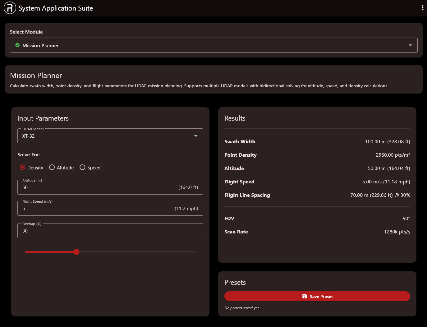
Purpose: The Mission Planner helps operators calculate the necessary flight parameters (altitude, speed, line spacing) to achieve specific LiDAR data quality goals (point density, overlap). It supports bidirectional solving for various LiDAR models.
How to Use
Select Module: Ensure Mission Planner is selected in the main module dropdown.
Choose LiDAR Model: under the “Input Parameters” section, select your specific LiDAR sensor from the LiDAR Model dropdown menu (e.g., XT-32).
Select Solve Target: Determine what variable you want the system to calculate by choosing one of the Solve For radio buttons:
Density: Calculate required altitude/speed to meet a target point density.
Altitude: Determine necessary altitude based on speed and density constraints.
Speed: Calculate maximum flight speed to maintain density at a given altitude.
Input Parameters: Enter the known constraints into the remaining fields:
Altitude (m): Flight height above terrain.
Flight Speed (m/s): Velocity of the aircraft.
Overlap (%): Desired sidelap between flight lines.
Note: The available inputs change based on your “Solve For” selection.
Review Results: As you adjust inputs, the Results panel on the right will update instantaneously.
Pay attention to:
Swath Width: The ground coverage of a single scan line.
Point Density: The estimated points per square meter.
Flight Line Spacing: The required distance between parallel flight lines to achieve the specified overlap.
Save Presets (Optional): If you frequently use specific setups, click the Save Preset button at the bottom right to store the current configuration for future use.
3. LiDAR Scan Diagnostics Module #
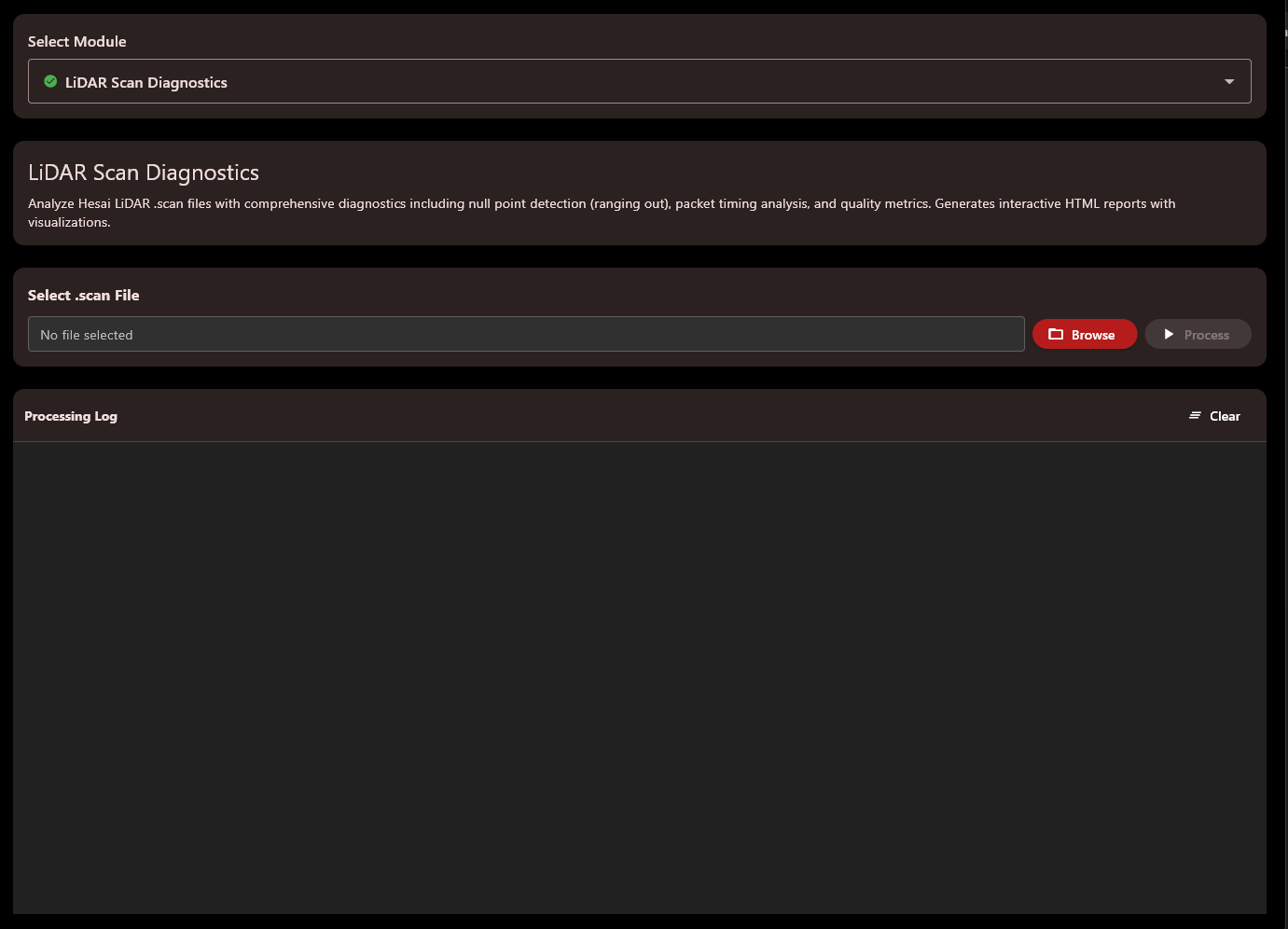
Purpose: This module is used post-mission to analyze XT32, and XT32-M2X LiDAR .scan files. It checks for null points, packet timing issues, and other quality metrics, generating interactive HTML reports.
How to Use:
Select Module: Choose LiDAR Scan Diagnostics from the main dropdown.
Load Data: In the “Select .scan File” section, click the Browse button. Navigate to and select the .scan file you wish to analyze.
Start Processing: Once the file path is loaded into the text field, click the Process button.
Monitor Progress: The Processing Log panel at the bottom will display the status of the analysis. Once complete, the log will indicate where the interactive HTML report has been saved.
Clear Log: Use the Clear button at the top right of the log panel to reset the view for subsequent operations.
4. MavLink Simulator Module #
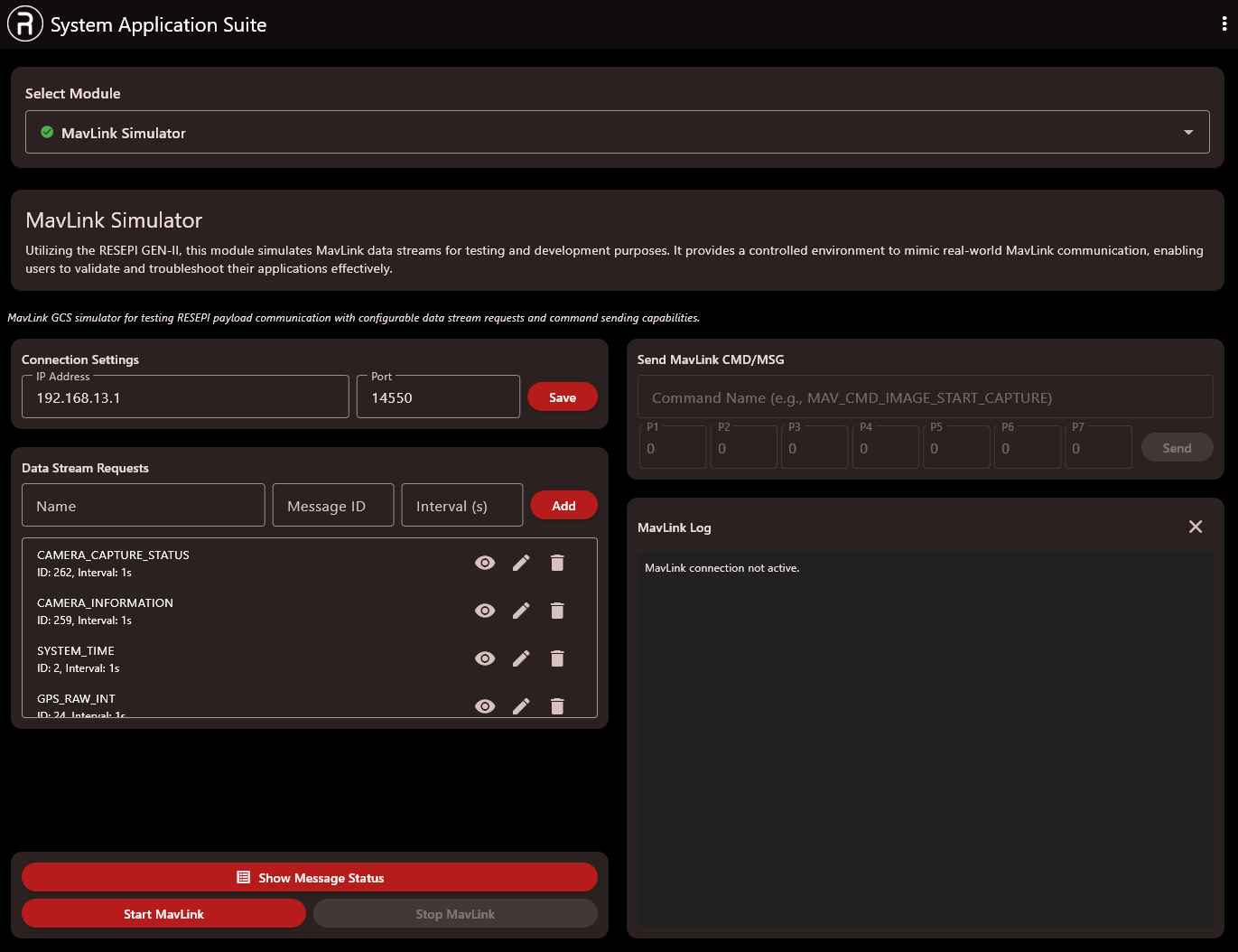
Purpose: Designed for developers and integrators, this module simulates MavLink data streams (mimicking systems like RESEPI GEN-II). It is used to validate and troubleshoot GCS connections and application responses in a controlled environment.
How to Use:
Select Module: Choose MavLink Simulator from the main dropdown.
Connection Settings:
Enter the target IP Address and Port for the MavLink connection.
Click Save to apply these settings.
Configure Data Streams:
Under “Data Stream Requests,” define the streams you want to simulate by entering a Name, the specific Message ID, and the desired Interval (s).
Click Add to include it in the active list below.
Tip: Use the eye icon to hide/show streams, the pencil to edit, and the trash can to delete them.
Send Commands (Optional):
Use the “Send MavLink CMD/MSG” section to manually send specific commands.
Enter the Command Name and any necessary parameters (P1-P7).
Click Send.
Start Simulation: Click the red Start MavLink button at the bottom left to begin streaming data.
Monitor Status: The MavLink Log panel on the right will show connection status and activity. You can also click Show Message Status for detailed stream metrics.
5. Image Processing Module (GPS EXIF Writer) #
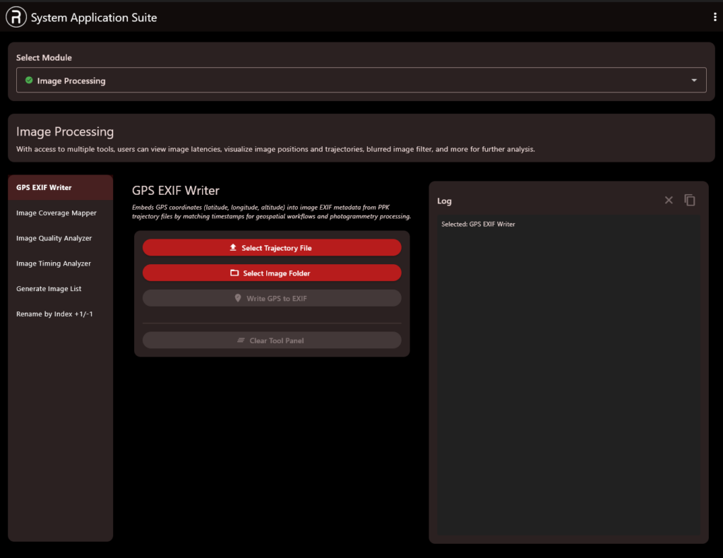
Purpose: The Image Processing module contains various tools. The tool shown, GPS EXIF Writer, is used to embed precise GPS coordinates (latitude, longitude, altitude) into image EXIF metadata by matching image timestamps with a PPK trajectory file.
How to Use:
Select Module: Choose Image Processing from the main dropdown.
Select Tool: Ensure GPS EXIF Writer is selected in the left-hand sidebar menu.
Load Trajectory: Click the Select Trajectory File button and locate your post-processed kinematic (PPK) trajectory file (often a .txt or .pos file).
Load Images: Click the Select Image Folder button and choose the directory containing the images you wish to geotag.
Run Process: Once both inputs are loaded successfully, the Write GPS to EXIF button will become active. Click it to start the geotagging process.
Review Log: The Log panel on the right will display progress and confirm when the images have been successfully updated with GPS data.
6. System Diagnostics Modules (RESEPI LITE & RESEPI GEN-II) #
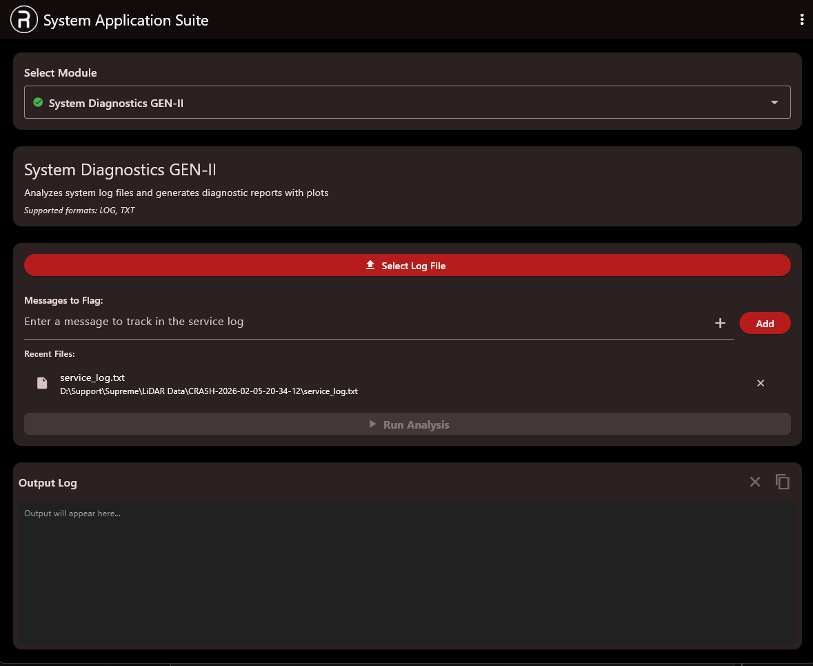
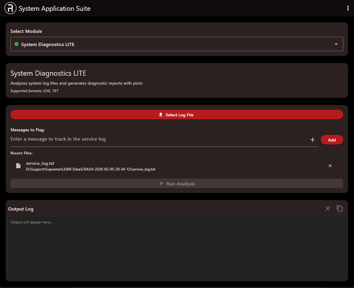
Purpose: These modules analyze system log files (supported formats: LOG, TXT) to generate diagnostic reports containing plots. They are essential for troubleshooting system crashes or performance issues. Note: The workflow is identical for both the “LITE” and “GEN-II” versions shown in the images.
How to Use:
Select Module: Choose either System Diagnostics LITE or System Diagnostics GEN-II from the main dropdown depending on your hardware generation.
Select Log File: Click the large red Select Log File button at the top to browse for the log file you wish to analyze.
Use Recent Files: Alternatively, if you have analyzed files recently, they will appear in the “Recent Files” list. Click on a file path to load it quickly.
Flag Messages (Optional): If you are looking for specific events, enter keywords into the “Enter a message to track…” field and click Add. The analysis will highlight these events.
Run Analysis: Once a log is selected, the Run Analysis button at the bottom of the main panel will become active. Click it to begin.
View Output: The results of the analysis will be generated, and process information will appear in the Output Log panel at the bottom.