Pix4DMatic – Using RESEPI to Make Othomosaic

RESEPI User Manual

Tutorials and Supporting Documents

Images to Orthomosaic #

Orthomosaic is commonly implemented geospatial deliverable created using images. This guide will show how to retrieve these models from an images from RESEPI in PIX4Dmatic by PIX4D. We will also look at the key aspects to pay attention to.

Data Preparing #

After processing LiDAR data in PCMasterPro, the project folder will look like this, Figure 1.

Figure 1. Folder with data after processing in PCMasterPro.

We will need a folder of photos named “Camera.” It contains all the photos captured during the mission. In addition, please note the file “ppk_imageList_p4d.csv,” which contains the camera’s coordinates and orientation angles—information that is essential for data processing (to create this file, you’ll need to save the colored point cloud in PCMasterPro). It’s also important to have a file with Ground Control Points (GCPs) for georeferencing. The more accurately the GCPs are measured, the more accurate the georeferencing of the orthomosaic will be.

Import images and Project Setup #

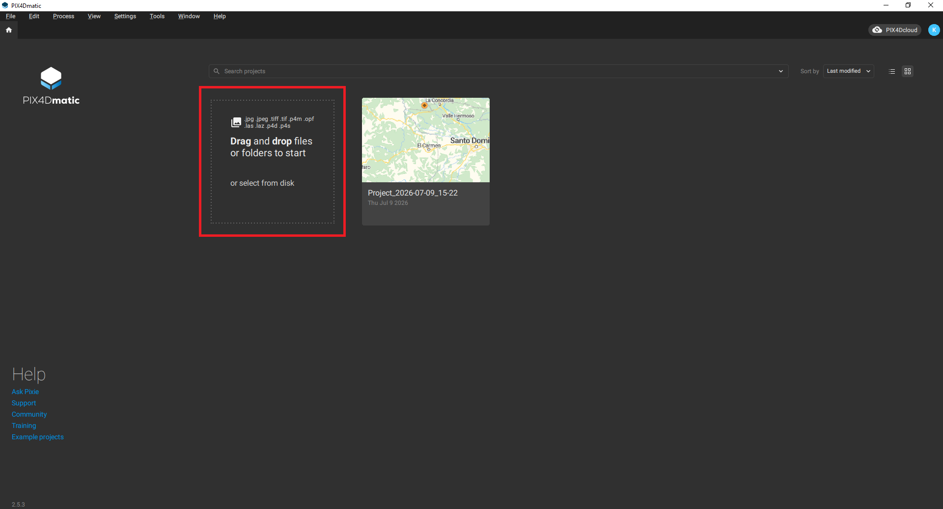
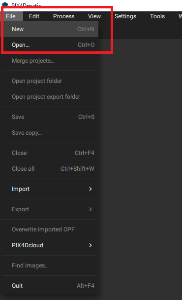
To generate an orthomosaic, you need to create a project and import images. To do this, click on the area highlighted by the red border in the program’s startup window, as shown in Figure 2. Alternatively, you can use the “Project” -> “New” menu, as shown in Figure 3.

Figure 2. The program's start window.
Figure 3. Creating a project via menu items.

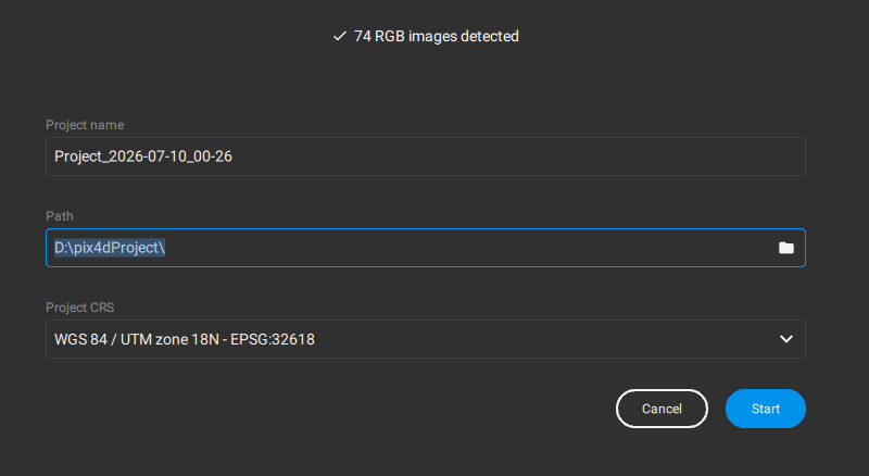
We’ll select the entire project folder, and the program will automatically find and count the number of photos. After that, the interface will change, as shown in Figure 4. Here, you’ll need to enter a project name and the path where the project will be saved.

Figure 4. Name and path to project files.

The program also automatically determined the project’s coordinate system based on information from the images, so we’ll leave this setting unchanged. After configuring the settings, click “Start.”

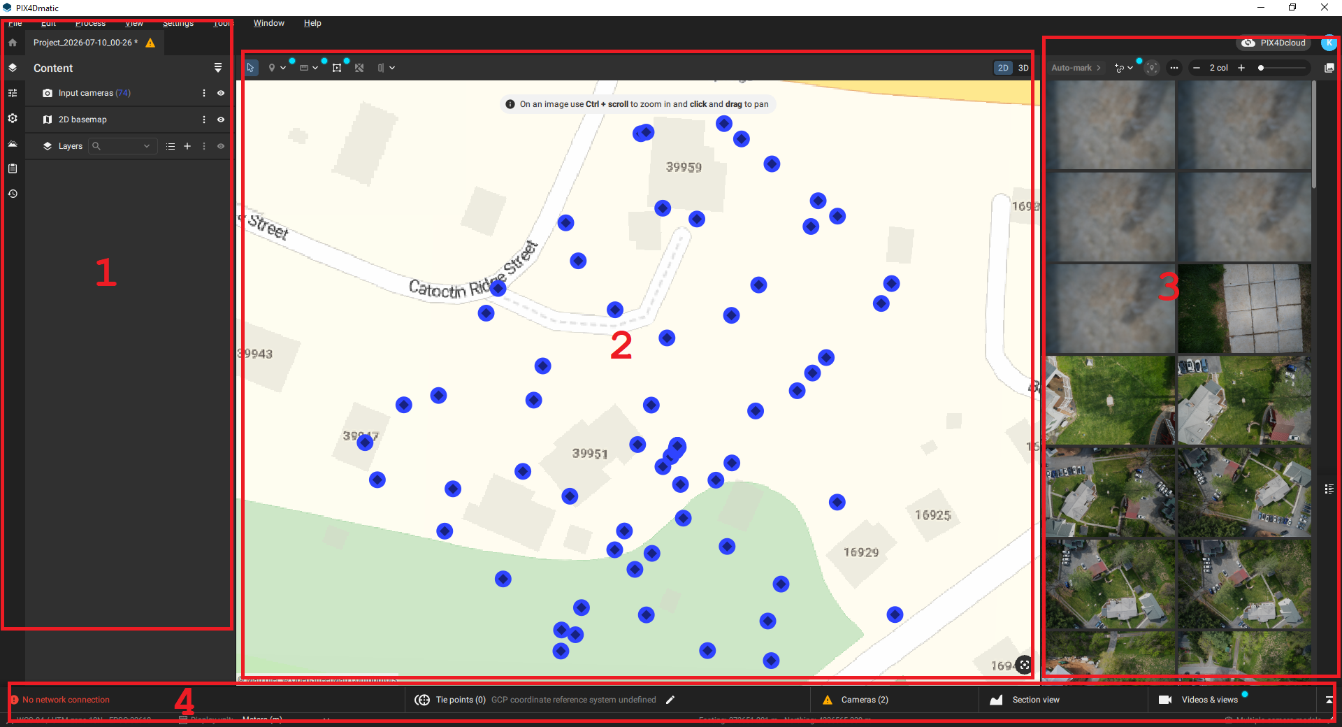
The program window will appear as shown in Figure 5. The window can be divided into four areas:

1 – Area for selecting the mode and processing parameters.
2 – Map display area. The blue circles indicate photos taken during the mission. Clicking on them will automatically select the corresponding photo in the image editing area (3).
3 – Image editing area. Here, we will match our GCPs with the ground markers in the photos.
4 – Area for working with GCPs and the camera.

Figure 5. The main program window after setting up the project.

Data Processing #

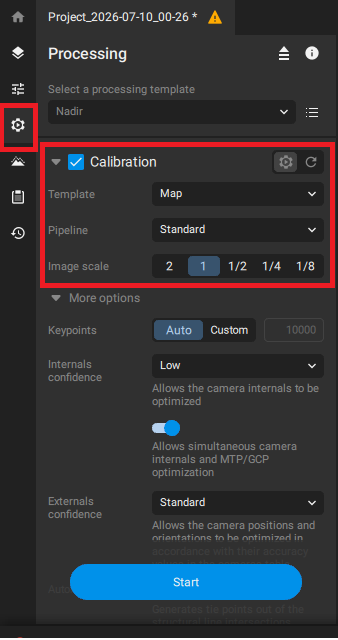
Before starting processing, you need to run the calibration procedure. To do this, click the gear icon in the settings panel, check the “Calibration” box, and select the calibration settings as shown in Figure 6 (the settings are shown for demonstration purposes only; you can change them as you see fit, depending on the project and the desired result).

Figure 6. Processing Options menu.

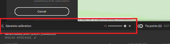
The status bar will display the status of the calibration process, as shown in Figure 7.

Figure 7. Status bar
Figure 7. Status bar.
Once the process is complete, click the “Camera” tab to open a list of images, as shown in Figure 8.
Figure 8. The list of images.
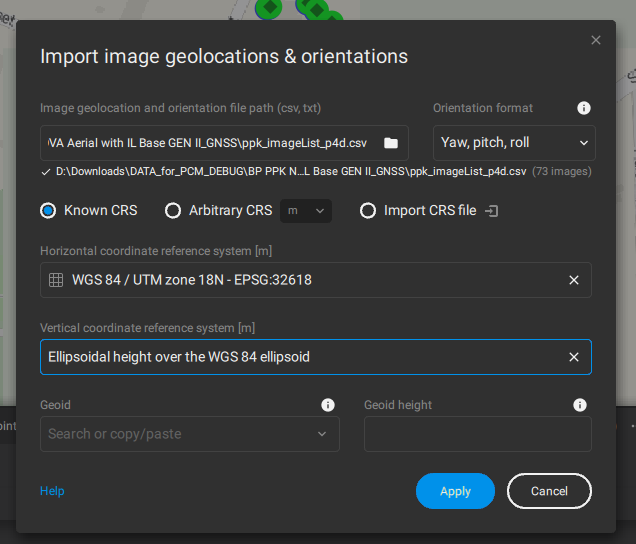
Please note that some fields are empty because the EXIF data contained in the images is incomplete. To fix this, click the three dots next to the “Camera” tab and select “Import image geolocations and orientations…” from the drop-down menu. A window will open, as shown in Figure 9.
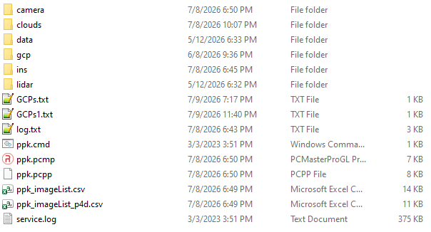
Figure 9. “CSV/txt” File Selection Window.

Select the file “ppk_imageList_p4d.csv,” specify the orientation format as “Yaw, Pitch, Roll,” and select the horizontal and vertical coordinate systems. Click “Apply.” The information in the list will then be updated. Next, we’ll add control points for georeferencing the images.

Adding Ground Control Points #

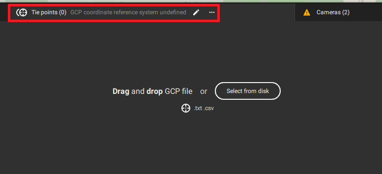
  • To add control points, click the icon with the crosshairs in the “Tie points (0)” tab, Figure 10.
Figure 10. GCP Addition Tab.

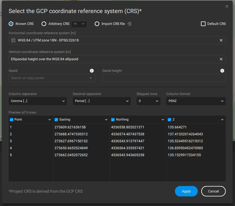
Click “Select from disk” and select the file containing the control points. A window like the one shown in Figure 11 will open. Select the coordinate systems (if the program does not detect them automatically) and specify the “Column format.” In our case, it is “Point number, Easting, Northing, Z.”.

Figure 11. «GCP Manager» window.

Click “Apply.”

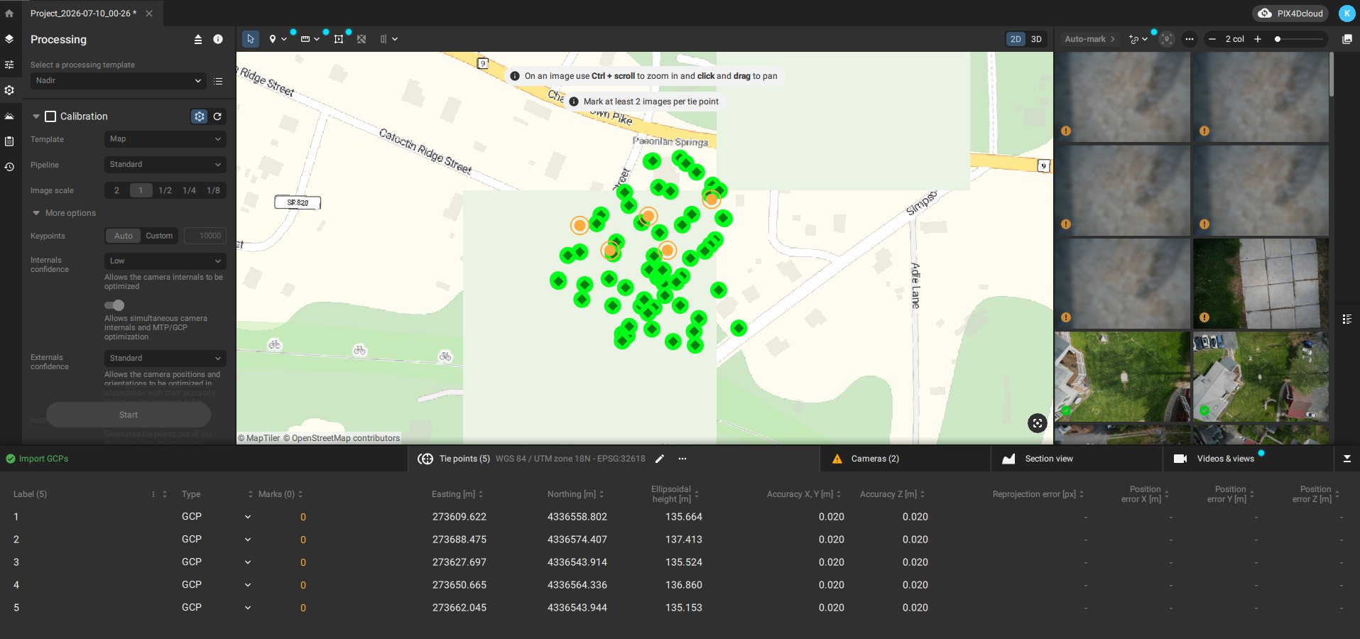
The list of points will be updated and they will appear in the map view window, as shown in Figure 12.

Figure 12. The program window after adding GCPs.
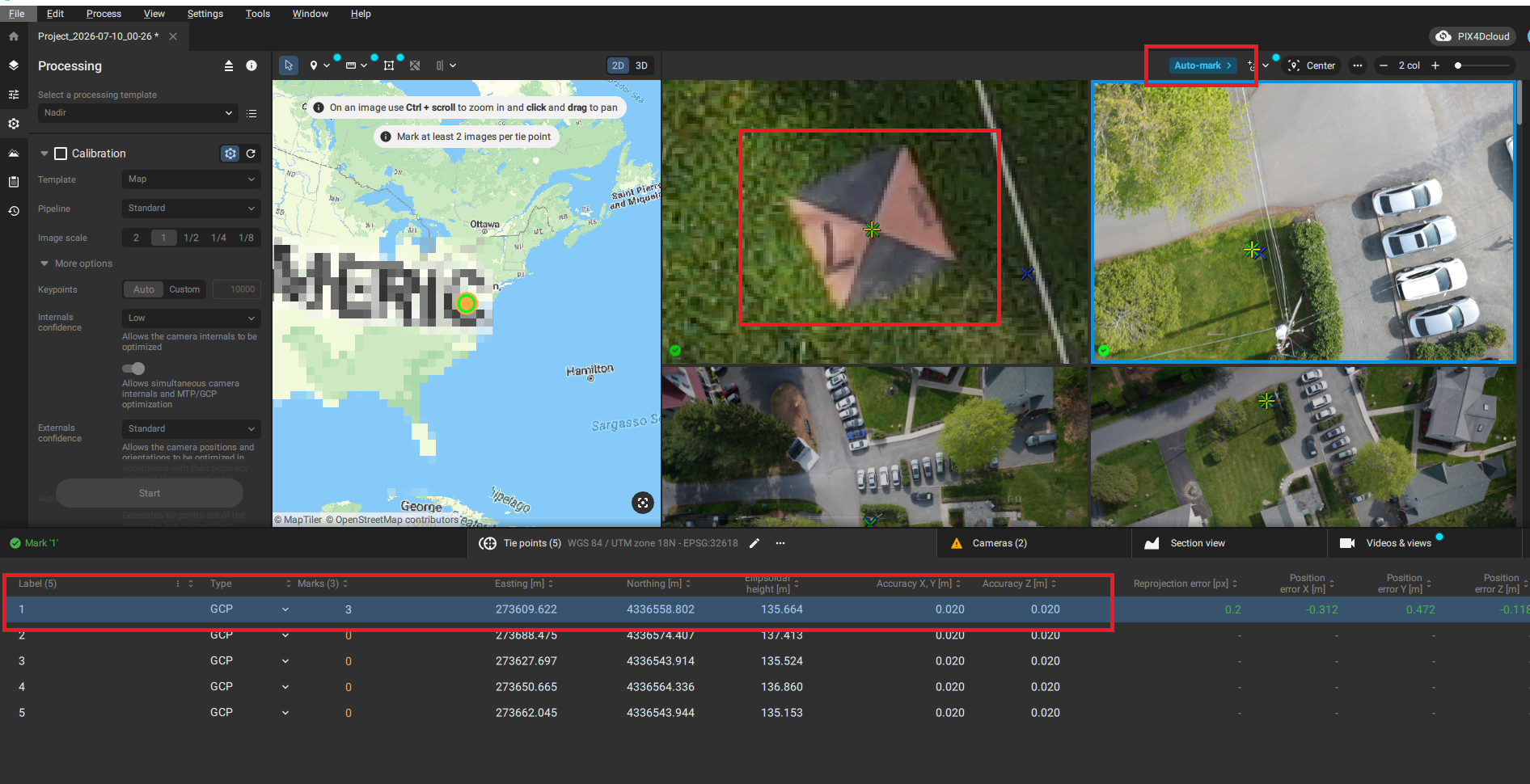
  • For each control point, you need to select 2–3 photos with the corresponding marker. For example, we know that the first control point corresponds to target number 7. Click on the first control point in the list, then on a photo in the photo list, and locate the target in the photos (you can zoom in and pan the photo as needed). It is sufficient to mark 2–3 photos where the target appears. Click in the center of the target with the left mouse button (we recommend zooming in on the photo to ensure the click is exactly in the center of the target). A yellow and green cross will appear, Figure 13. After marking 2–3 photos, you can click “Auto-mark,” and the program will automatically detect the corresponding target in all photos where it appears.
Figure 13. Selecting markers based on GCP numbers.
  • Repeat the procedure for the remaining control points.
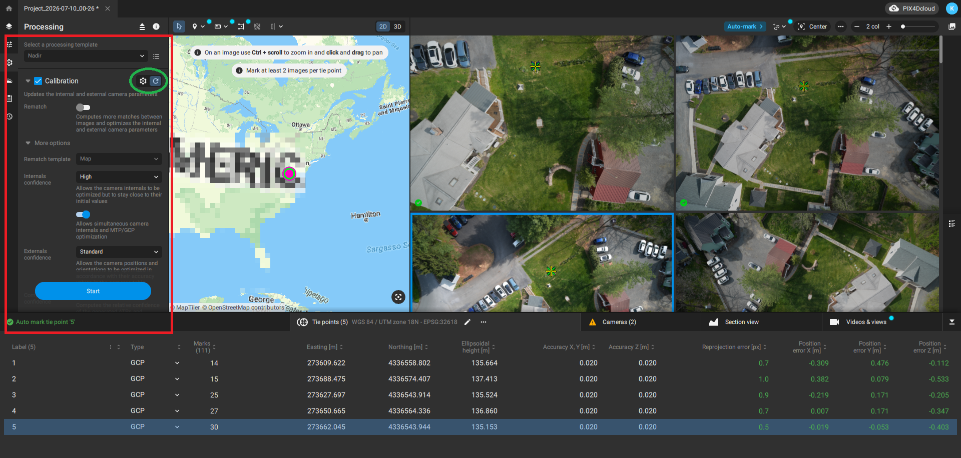
  • Next, in the “Processing” tab, select “Calibration” in “Reoptimization” mode (click the curved arrow next to the gear icon), Figure 14. This tool will correct the georeferencing errors in the images.
Figure 14. “Reoptimize” mode.

Select the parameters and click “Start.” Once the process is complete, the error has decreased significantly, as shown in Figure 15.

Figure 15. Program Window After Reoptimization.

After georeferencing the data, we can run the data processing to generate a DSM, an orthomosaic, and a point cloud.

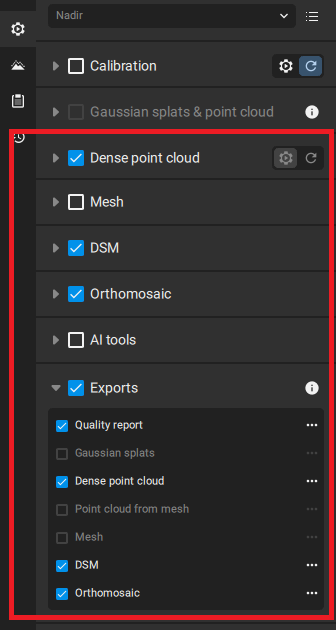
  • To do this, click “Processing” and check the boxes next to “Dense Point Cloud,” “DSM,” and “Orthomosaic,” as shown in Figure 16. Leave the processing parameters as they are (if necessary, you can adjust them to achieve the best results by reprocessing the data and analyzing the reports). Don’t forget to check the “Export” box to save the result to disk. Click “Start” and wait for processing to complete.
Figure 16. Processing Options.

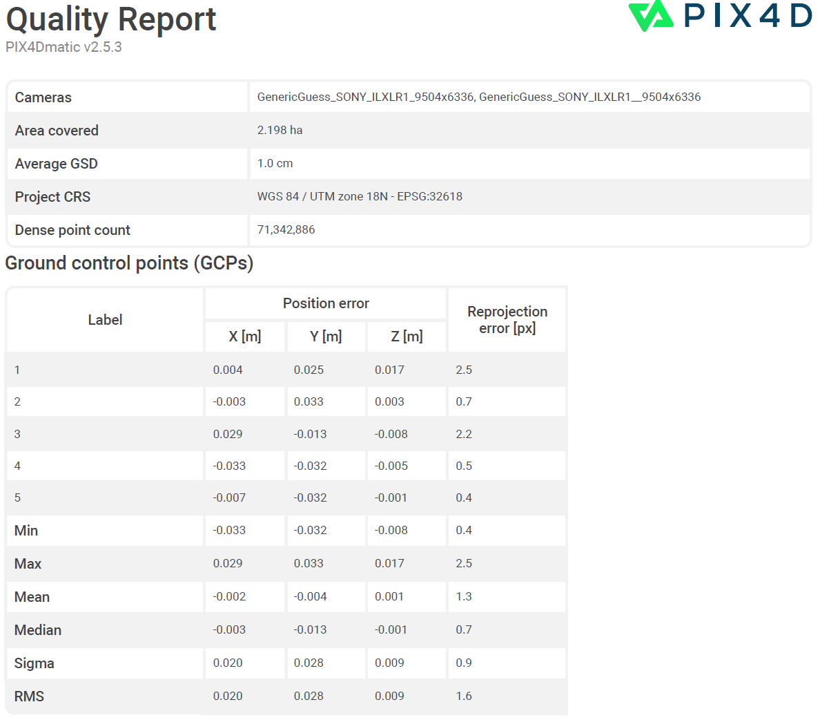
Now, the folder we selected for this project will contain the point cloud, DSM, and orthomosaic files, as well as a report. In the report, we can see the georeferencing accuracy results, as well as the Average GSD, as shown in Figure 17. As you can see, we achieved an excellent result: the average GSD is 1 cm, and the RMS georeferencing error is less than 3 cm.

Figure 17. Quality Report.

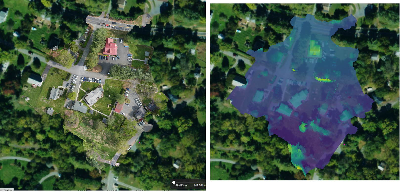
As a result, we obtained an orthomosaic and a DSM with precise georeferencing, which we overlaid on a Google Map (Figure 18).

Figure 18. Result of data processing.